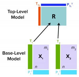
Figure 1: Hierarchical model schematic; information from all base-level models is communicated to a top-level model through their respective matrices (Tj) into a consensus matrix R. R is used to further summarize data from all base-level models by generating top-level scores TTL and loadings PTL.
Purification is an essential process in biopharmaceutical manufacturing that separates a therapeutic protein in its active form from impurities. A typical purification process consists of several chromatography unit operations, and each unit operation comprises multiple phases. During the operation of each step, continuous (time-series data per parameter for each batch) and batch data (one data point per parameter for each batch) are generated by in-line sensors installed in chromatography skids on the production floor and with at-line/off-line in-process samples, respectively. Such process data can be leveraged for developing advanced data-driven models that can provide insights for process experts and support their decisions and actions.
Traditionally, control charts for in-, on-, at-, and off-line analyses are trended univariately (one parameter per chart) to monitor a biomanufacturing process. That approach requires a review of multiple charts at the same time to find all correlations among the parameters during real-time or retrospective analysis. That makes root-cause analysis and early fault detection time consuming and cumbersome.
Trying to find relationships among multiple attributes by simply reviewing individual charts for each parameter could be exceptionally challenging and limited. Multivariate data analysis (MVDA) is a methodology comprising advanced statistical techniques that can be used to analyze large, complex and heterogeneous data sets at the same time. The development and use of such MVDA models would provide for effective and efficient near-real-time process monitoring and early fault detection and diagnosis.
MVDA models can be used to monitor multiple process variables with a few multivariate metrics while leveraging useful process information found in the correlation structure between process variables. Thus, MVDA is a powerful methodology that can be used to assist process engineers and scientists with root-cause identification for process excursions. It also can provide numerous insights into manufacturing operations that in turn can be leveraged to enhance overall process understanding and control.
The case study below highlights an application of advanced data-driven modeling to an affinity-chromatography column in commercial biologics manufacturing. Researchers developed a multivariate model using process parameters and in-process control parameters at the purification step and visualized the correlation among them. We also present the application of a hierarchical data-driven modeling methodology for effective monitoring of a purification unit operation and its corresponding phases and highlight the utility of such data-driven models. Finally, we overview the key steps involved in developing advanced, data-driven models in biologics manufacturing.

Figure 2: In this cross-validation protocol, the data set is partitioned into training and testing subsets. Models are developed for each cross-validation round (with different partitioning of a data set). Cross-validation outcomes from all models are averaged to estimate a model’s final predictive power.
Materials and Methods
Purification Process: In bioprocessing of recombinant therapeutic proteins, purification takes place downstream of cell culture and isolation steps. A recombinant protein is separated from a pool of other proteins during cell culture. Different chromatography columns are used for purification, depending on the type of protein being purified. Ion-exchange (IEX), hydrophobic-interaction (HIC), and affinity chromatography are among the most widely used separation techniques. Purification usually is divided into several phases such as equilibration, load, wash, elution, and regeneration and storage of the column.
Below, we discuss multivariate models developed for on-line monitoring of a therapeutic protein purification process using an affinity-chromatographic column. This column has peptide ligands (with target-protein binding domains) on stationary-phase beads that capture target-protein molecules during the load phase and releases them in elution. Nontarget proteins without an affinity for the column ligands flow through the column as waste material.
A purification column is equilibrated with respect to its internal pH and conductivity before loading a target protein. Flowing through a buffer ensures that the conditions in a column are appropriate to handle that protein.
During column loading, therapeutic-protein molecules with affinity to packed beads within the column bind to those beads. Impurities flow through the column to waste because they have no affinity for peptide ligands.
Wash buffer is passed through a column to dislodge only loosely bound impurities while keeping tightly held target protein molecules attached to stationary-phase beads.
Elution buffer is passed through a column to disrupt the bonds between a target protein and peptide ligands and to facilitate dislodging target-protein molecules from the column. Eluate containing a target protein is collected for further processing.

Figure 3: In the data structure, (left) for batch-evolution models, differently colored data sets represent data from different batches. Each data set comprises m number of X process-related variables, n observations (time points), and one Y variable (column volume). (right) For batch-level model, data-set columns used for batch-evolution models are transposed to generate the data set for batch-level model. Each row represents a different batch. X1time1 denotes the value of first X1 variable at time1. Similarly, Xmtimen denotes value of Xm variable at timen.
Data and Data Sources: Data are the foundation of modeling. Two types of data are used to develop MVDA models for an affinity-chromatography column: in-line/on-line data and at-line/off-line data.
In-Line/On-Line Data: The following types of in-line measurements are used in the model: totalized volume of effluents from a chromatography column, conductivity, UV absorbance, temperature, pressure, and flow rate. Data from process measurements are stored in a database called PI process historian (from OSIsoft). All time-series data obtained from process sensors (e.g., conductivity sensors) are historized in the PI Data Archive component. The corresponding batch context (e.g., batch identification number, individual process phase start and end timestamps) is stored in the PI Asset Framework (AF) database.
At-line/Off-line Data: Both at-line and off-line data are accessible through the Discoverant relational database (from BIOVIA). Structured Query Language (SQL) (developed by IBM) is used to retrieve data from underlying data systems such as manufacturing execution systems (MES), laboratory information management systems (LIMS), and Systems Applications and Products (SAP) software. The types of at-line and off-line data used for model development include protein solution (bulk) attributes, bulk thaw process attributes, column load attributes, column attributes, eluate attributes, and sample measurements.
Software: For modeling, researchers used Simca 14.1 (from Sartorius Stedim Biotech) and Matlab 2015b (from MathWorks) software. Matlab Python 3.6 software (from Python Software Foundation) was used for data acquisition, preprocessing, visualization, and model automation.
In-Line Data Preprocessing: In- and on-line data obtained from the PI process historian must be processed in a standardized way to remove obvious abnormalities (e.g., chromatogram baseline offset) while capturing data and to align the data to a standard form to facilitate batch-to-batch comparison. Data preprocessing for the purification step requires interpolation, segmentation, and alignment.
In-line data captured by different sensors during the progress of a batch are saved in the PI historian at an uneven sampling frequency for different process parameters. To monitor how all batches progress through purification and compare their performances, in-line data are interpolated for all parameters at a defined frequency.
Metadata (including start and end timestamps) for each phase in a batch for the affinity column were leveraged to segment in-line data into the corresponding phases. Continuously recorded time-series data were extracted between the start and end time points. Time-series data for each column sensor were preprocessed to ensure that all batches aligned with respect to the start time of every subphase of the affinity purification process.

Figure 4: In this purification column monitoring model structure, the lowest level in the hierarchy is the batch-evolution model (BEM), which is a partial least squares (PLS) model with in-line data only. The middle level consists of batch-level models (BLMs) for phases that are principal component analysis (PCA) models with in-line and at-line/off-line data. Finally, the top-level model is a comprehensive PCA model comprising in-line and at-line/off-line data for all phases taken together.
MVDA statistical techniques and algorithms are used to analyze data from more than two variables. MVDA can be used to detect patterns and relationships in data. Some applications include clustering (detection of groupings), classification (determining group and class membership), and regression (determining relationships between inputs and continuous numerical outputs). Some widely used MVDA techniques are principal component analysis (PCA) and partial least squares (PLS) projection to latent structures.
PCA can be used to obtain an overview of underlying data without a priori information. It is used to label and map those data to target or output values (1). PCA also is used to find structure and patterns in data by reducing the dimensionality of data sets in which collinear relationships are present. The working principle of PCA is to summarize original data by defining new, orthogonal, latent variables called principal components (PCs).
PCs consist of linear combinations of original variables in a data set. They are chosen such that the variance explained by a fixed number of PCs is maximized. The values of the original data in the new latent variable space are called scores. Given a data set described by an n × m matrix X with n observations and m variables, T denotes a n × k matrix containing the k PC values called scores. The coefficients pjq with j = 1, . . . m and q = 1, . . . k that determine the contribution of each individual variable Xij with i = 1, . . . n to the principal component are called loadings. The m × k matrix P is called a loading matrix, and the relationship among T, X, and P is given in matrix notation by the following equation: X = TPT + E, where E denotes the residual n × m matrix. The residual contains variance not explained by the PCs 1, . . . k. Basilevsky provides an in-depth introduction to PCA (1).
Model quality is assessed with cross-validation and external data sets, if available. To that end, the R² and Q² statistics are evaluated. The R² statistic describes the fraction of the sum of squares explained by a model, and the Q² statistic conveys information about the predictive ability of a model (2).
PLS regression is used to determine functional relationships between inputs and outputs (3, 4). This approach is similar to PCA in that regression is conducted not on the original variables available in a data set, but on fewer, orthogonal ones called latent variables. Those are linear combinations of original variables. Unlike with PCA, in which latent variables are chosen to maximize variance, latent variables in PLS are determined such that they maximize the covariance between dependent and independent variables. The following operations are conducted both in the x-space and the y-space to obtain a solution to a regression problem. In the x-space, a linear transformation is defined such that T = XW* and X = TPT + E with T denoting the x-scores matrix, P denoting the x-loadings matrix, W* denoting the x-weights matrix, and E denoting the x-residuals n × m matrix with k < m.
In the y-space, a transformation is sought such that Y = UCT + G, with U denoting the y-scores n × k matrix, C denoting the y-weights q × k matrix, G denoting the y-residuals n × q matrix. The x-scores are selected to minimize the x-residuals E and to be good predictors of Y. The y-scores are chosen to minimize the y-residuals G. R² and Q² can be calculated for PLS models.
Hierarchical modeling facilitates combining data from different models (either PCA, PLS, or both). Typically, that summarizes information from different parts of a process that are not similar, but are interconnected. Hierarchical modeling can be used to combine different phases in an affinity-chromatography purification process such as equilibration, load, wash, and elution, all of which are executed sequentially to accomplish the specific purification goals for each phase.
Hierarchical MVDA models consist of multiple levels (5). Figure 1 shows an example of a two-level hierarchical model structure, with base-level (BL) and top-level (TL) models for a process with two phases (1 and 2) with data X1 and X2, respectively. BL models can be multiple in number and based either on PCA or PLS. They summarize input data by their latent variables (e.g., score matrices Tj). BL models also are described by their loading matrices, such as Pj for PCA models, where j indicates the different BL models. Information from both BL models (corresponding to data sets X1 and X2) are fed into to a TL model through respective score matrices T1 and T2 with dimensions n × k1 and n × k2. The number of observations is denoted by n, and the number of latent variables for the BL models for phase 1 and 2 are k1 and k2, respectively.
The TL model input is defined by the n × (k1 + k1) matrix R, consisting of the scores from both BL models. Specifically, the score matrices Tj from individual x-blocks are combined to form the consensus matrix R, which is used to calculate scores and loadings for the TL model. For a PCA TL model, the relationship between score matrix TTP, loading PTP, and R matrices is given by TTP = R × PTP, where R = [T1, T2].
Generally, kTL < (k1 + k1), which indicates that the MVDA hierarchical modeling structure facilitates compressing data from all different BL models. An important benefit of hierarchical models is that each data block such as X1 and X2 with different dimensions retains comparable contribution to the TL model. Even if T1 consists of fewer latent variables than T2(k1 < k2), hierarchical modeling treats score matrices from both BL models with similar weight.
Cross-validation is a model-testing technique used to assess whether underlying statistical relationships in data are general enough to predict a data set that was not used for model training. For cross-validation, a given data set is partitioned into training and testing subsets. A model is developed using the training data set and then evaluated against the testing subset. Several rounds of cross-validation are carried out (with different partitioning), leading to multiple parallel models (Figure 2). Outcomes from all parallel models are averaged to estimate the final predictive power of a given model. The main purpose of cross-validation is to reduce the chance of overfitting, a condition in which a model fits the training data set well but is not general enough to predict an independent data set reasonably well.

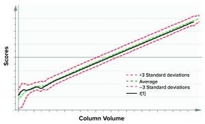
Figure 5: Batch-evolution model (BEM) score plot depicts scores of the first principal component for X as a function of column volume (considered as maturity variable for a purification process). The green dashed line denotes the mean of the data, and the red dashed lines correspond to ±3 standard deviations from the mean.
Results and Discussion
To make the MVDA purification-monitoring models discussed in this study a usable tool for end users, we considered the implementation of a meaningful modeling approach such that the model can detect process excursions. We also considered the benchmarking of new batches against historical batches. Thus, modeling was performed in two stages: model development and benchmarking.
Model Development: The development of an MVDA monitoring model for an affinity-chromatography column consists of three steps: model selection, model training, and model testing.
Model Selection: Evaluating batch trajectory for all phases of affinity chromatography (equilibration, load, wash and elution — henceforth referred to as phase) requires developing models that account for changes in in-line data as a function of batch progression. Such models are called batch-evolution models (BEMs) (2, 6).
Each phase can be evaluated further after batch purification by leveraging at-line and off-line data. Thus, an MVDA model is needed that can incorporate in-line time-series data and at-line and off-line discrete process parameters and attributes. Batch-level models (BLMs) can be used in this regard (2).
Finally, comprehensive evaluation of an affinity-chromatography operation requires the ability to evaluate all phases jointly. That objective can be achieved with a hierarchical modeling structure. Details of each level in the hierarchical model are described below.

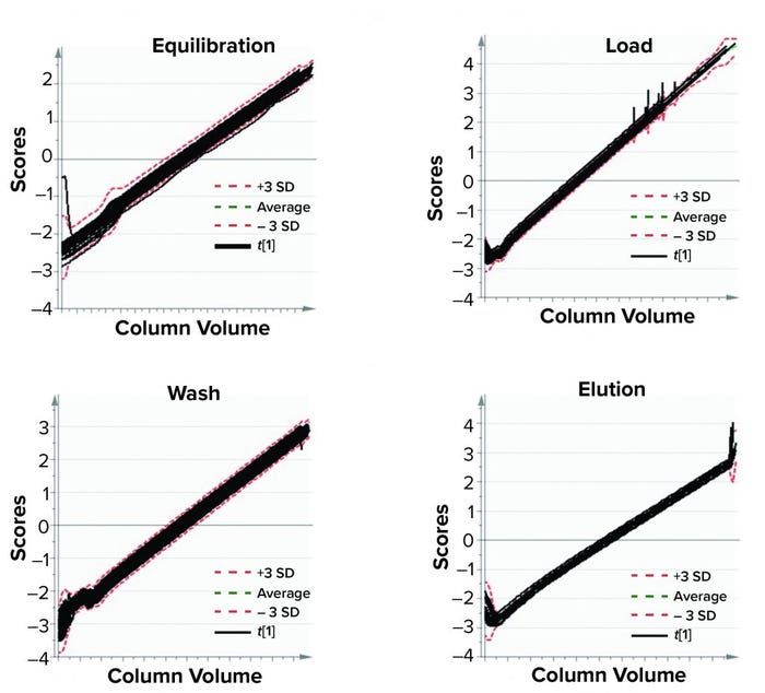
Figure 6: Model training; batch-evolution models were developed for different phases of a purification process. Each plot depicts batch progression summarized by the first multivariate data analysis score with respect to column volumes of material passed through a purification column. (SD = standard deviation)
BEMs are the first level in a hierarchical model structure. They provide an idea about how batches are progressing by taking into account in-line data for different process parameters (2, 6). Batch progression — either with respect to time of processing or volume of substance processed — is represented as a function of all available in-line process parameters, which are summarized by a few latent variables. BEMs are PLS models with process parameters as X variables and batch progression maturity as the Y variable. In this study, 11 in-line process parameters make up X variables, and column volume is used as variable Y. BEMs focus on maximizing covariance among all the process parameters X and batch maturity Y. The data sets used for generating BEMs contain time-series data for multiple batches. Each column in a data set corresponds to the different variables used for model development. Each row corresponds to different time points in measurement for that batch (Figure 3a).
BLMs make up the second level in a hierarchical model structure. They provide information about how a batch performed compared with previous batches. When a purification process is complete, a BLM takes into account in-line, at-line, and off-line data. In such cases, BLMs essentially are PCA models that focus on explaining the variations present in different process variables (2). All in-line time-series data are transposed such that each row in a BLM data set represents a single batch (Figure 3b).
TL models make up the third and highest level of a hierarchical model structure. They combine different levels in a multivariate modeling structure and provide a comprehensive view of the batch performance through all phases of purification process. Figure 4 shows all three levels.

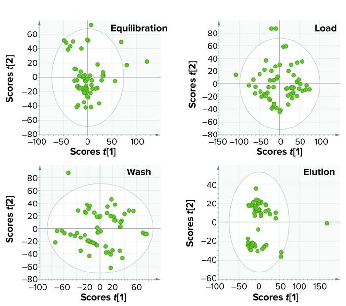
Figure 7: In model training of batch-level models for four phases of a purification process, each plot represents a single phase. The boundary of each ellipse indicates a 95% confidence of data used to build the models for each phase. Each circle within the ellipse represents a single batch, and all information about the batch was summarized for that particular phase by multivariate data analysis scores.
Model Training: After defining the structure of a model (in this case, a hierarchical structure with BEMs and BLMs at the base level and an overarching TL model), the next step is to train the model. Model training refers to the process of using historical data to define multivariate control limits that in turn would be the acceptable operating range. We used historical data consisting of sixty drug substance (DS) batches for model training in our study. All batches were considered for model training because they represent an acceptable operational range. Specifically, the quality of the final product was acceptable for release, so no batches were eliminated for model training.
Training a model with historical data (acceptable batches) requires defining multivariate control limits that are in fact the acceptable operational ranges. At the BEM level, the original time-series data are described with few latent variables, which can be visualized as a function of column volume. In Figure 5, the score plot of the first principal component of a single batch from BEM is shown as a function of column volume. The multivariate limits for BEMs are ±3 standard deviations (denoted by red dashed lines) of the historical data mean (shown as a green dashed line).
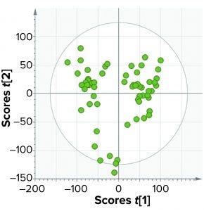
Figure 6 shows the BEM depictions for all purification phases and batches considered for model training. Most batches that were used for model training lie within the multivariate limits. To increase variability in the training data set (to reduce chances of overfitting), we included some batches that were outside the multivariate limit but had no process and product impact downstream of the purification process. Figures 7 and 8 show score plots for BLMs and TL model, respectively.

Figure 8: In model training, the top-level model of an affinity purification column takes into account four process phases: equilibration, load, wash, and elution.
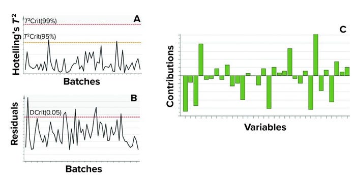
Process monitoring is facilitated using two multivariate metrics: the Hotelling’s T2 statistic and model residuals. The former represents the distance of an observation from the historical mean. The latter refers to the part of a data set that cannot be explained by a model (usually noise in the data or an occurrence not seen by the model before). Acceptable ranges of Hotelling’s T2 statistic and residuals for a batch is defined by the 95% critical level. If a batch lies within the acceptable range for Hotelling’s T2 statistic and/or residuals, no action is taken. However, if a batch lies outside those acceptable ranges for either or both metrics, then further investigation of contributing factors is triggered. Contribution plots provide a quantitative comparison of potential contributions for different process parameters toward a certain excursion. It depicts the difference of a selected batch or group of batches against the mean of all batches.
Figure 9 shows an example of the two excursion-detection metrics (Hotelling’s T2 statistic and model residual) and one diagnostic metric (variable contribution) for a single BLM. However, those values also were calculated for all BLMs (Figure 7) and for the TL model (Figure 8).
Model Testing: MVDA models are tested based on two objectives. The first objective is to ensure that the models developed using a training data set are general enough to describe an independent data set. For that, cross-validation is implemented. In our case, seven rounds of cross-validation were used for model testing. The second objective is to demonstrate a model’s ability to detect excursions and determine the underlying contributing parameters. Eleven additional batches for the affinity chromatography process have been used to detect process excursions and for model benchmarking.

Figure 9: In this example of model metrics used for excursion detection and diagnosis for a single batch-level model, (a) Hotelling’s T2 statistic and (b) model residuals both are used to identify excursions during process monitoring. (c) Contribution charts denote contributions of variables toward an excursion for a batch, compared with the mean of all batches.
Model benchmarking refers to the evaluation of new batches (batches that are not used for model training) against historical expectation, which represents an acceptable operational range for a process. That evaluation enables the assessment of potential excursions and investigation of the identified contributing factors.
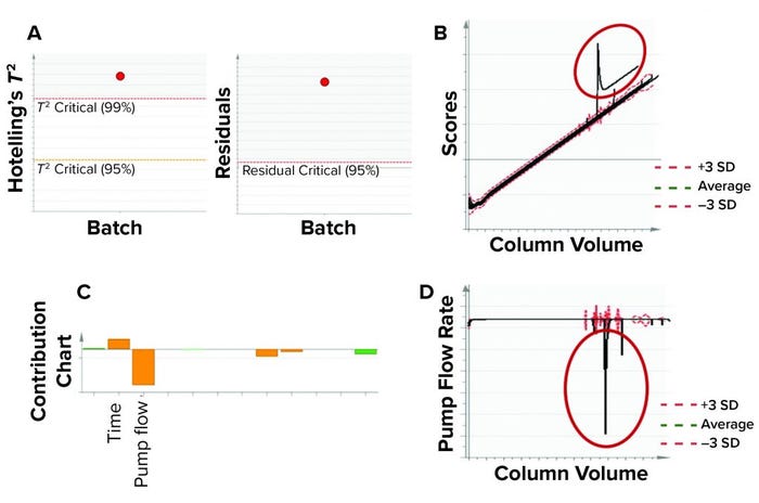
Eleven purification batches that were not included in training data set were used for model benchmarking. That served as a test for our model’s ability to detect excursions. We used Hotelling’s T2 statistic and model residuals multivariate metrics for evaluating batches. Figure 10 shows an example of model testing and benchmarking. A process excursion was detected for one batch in both the Hotelling’s T2 statistic and model residuals values (both being outside the acceptable levels) for the affinity chromatography column. The excursion was confirmed in the MVDA score space for the loading phase BEM.
As Figure 10c shows, pump flow rate had the highest contribution to this excursion. Further investigation into the univariate plots showed that the pump was stalled for some time during the load phase (Figure 10d). Subject-matter experts from our manufacturing sciences and technology department also confirmed that the pump was stalled because of some technical issues during the load phase. Thus, through this monitoring procedure, excursions could be detected that might influence product quality.

Figure 10: In this model benchmarking example, the model detected an excursion using multivariate data analysis (MVDA) metrics and identified contributing process parameters using a contribution chart. (a) Process excursion detected for a batch through MVDA metrics Hotelling’s T2 statistic and residuals in load-phase batch-level model (BLM). (b) Excursion was confirmed by MVDA score plot of load-phase batch-evolution model. (c) A contribution chart was used to identify process parameters associated with the excursion, and the column pump flow rate had the highest contribution to this excursion. (d) Univariate representation shows pump flow rate and column volume. Column-loading pump flow rate was significantly lower for some time during the load phase of the batch because of pump stalling for a period of time. (SD = standard deviation)
Developing Effective Models
A large amount of process and product data are generated during commercial biomanufacturing. Those large and complex data sets typically come from in- and on-line sensors for various unit operations as well as from benchtop analyzers on the production floor and quality control laboratories. Herein, we focused on how the wealth of manufacturing data for a purification process can be used to develop advanced data-driven models that can be leveraged to generate insights for process experts and used to support organizational decisions. The case study presented was for preparative affinity chromatography used in the manufacture of a recombinant therapeutic protein.
The multivariate models developed for an affinity chromatography column provided effective and efficient in- and on-line process monitoring using available in-, on-, at-, and off-line data. The study included a multivariate hierarchical modeling approach to account for several purification phases of the affinity chromatography operation and to facilitate comprehensive assessment.
Results showed that a hierarchical model can monitor the trajectory of process parameters for every process phase in addition to a joint evaluation of process parameters with in-process controls. Specifically, individual BEMs and BLMs were developed for each phase, enabling researchers to evaluate a new batch’s progression in the context of historical expectation.
Available historical data were leveraged for training those models, and additional data were used for model testing and benchmarking. The developed models describe historically accepted operating conditions for evaluating new batches. Benchmarking can be performed with a few multivariate diagnostics and contribution analyses, which highlight factors (original variables) potentially contributing to excursions. Models presented herein were tested and shown to be capable of detecting excursions.
Our case study demonstrates how the development of advanced, hierarchical, data-driven models enables the effective purification process monitoring through a comprehensive assessment of all phases of a unit operation. The models also detected patterns and relationships within each phase and across them. Multivariate modeling also ensures efficient process monitoring because a large number of process parameters can be evaluated by using only a few multivariate metrics. This modeling approach also can be applied to multiple unit operations in biomanufacturing; they are not limited to purification alone. Developing multivariate models for cell culture, viral inactivation, and final product manufacturing (fill–finish) processes also can provide process understanding, an efficient method of process monitoring, and early fault detection.
Advanced, multivariate, data-driven modeling can enhance process monitoring for early fault detection and fault diagnosis for purification unit operations. It simultaneously supports overall organizational efforts for process understanding and control of a biologics manufacturing process.
Acknowledgments
The authors thank all colleagues from the Manufacturing Sciences and Technology department who supported this work.
References
1 Basilevsky A. Statistical Factor Analysis and Related Methods: Theory and Applications. John Wiley & Sons: Hoboken, NJ, 2009.
2 Eriksson L, et al. Multi- and Megavariate Data Analysis: Basic Principles and Applications. Umetrics Academy: Umeå, Sweden, 2013: 425.
3 Wold S, et al. The Collinearity Problem in Linear Regression: The Partial Least Squares (PLS) Approach to Generalized Inverses. SIAM J. Sci. Stat. Comput. 5(3) 1984: 735–743; https://doi.org/10.1137/0905052.
4 Wold S, Sjöström M, Eriksson L. PLS Regression: A Basic Tool of Chemometrics. Chemometr. Intell. Lab. Syst. 58(2) 2001: 109–130; https://doi.org/10.1016/S0169-7439(01)00155-1.
5 Rännar S, MacGregor J, Wold S. Adaptive Batch Monitoring Using Hierarchical PCA. Chemometr. Intell. Lab. Syst. 41 (1) 1998: 73–81; https://doi.org/10.1016/S0169-7439(98)00024-0.
6 Wold S, et al. Modeling and Diagnostics of Batch Processes and Analogous Kinetic Experiments. Chemometr. Intell. Lab. Syst. 44(1–2) 1998: 331–340; https://doi.org/10.1016/S0169-7439(98)00162-2.
Shreya Maiti is a senior scientist, and corresponding author Konstantinos Spetsieris is head of data science and statistics, both at Bayer US LLC, 800 Dwight Way, Berkeley, CA 94710; 1-510-705-4783; [email protected]; http://www.bayer.com.
