HTTPS://STOCK.ADOBE.COM

The 2011 process validation (PV) guidance document from the US Food and Drug Administration (FDA) states that the number of samples used for PV “should be adequate to provide sufficient statistical confidence of quality both within a batch and between batches. The confidence level selected can be based on risk analysis as it relates to the particular attribute under examination” (1). In alignment with those expectations, I present herein two statistical methodologies for calculating the necessary number of process performance qualification (PPQ) runs: the tolerance interval (TI) method and the process performance capability (PpK) method. Both entail the following sequence of steps for demonstrating that the PPQ results obtained have an acceptable statistical confidence:

1: Assess the risk of an attribute/parameter to be monitored.

2: Assess statistically the reliability for the sample size of data used to gain process knowledge.

3: Define targeted statistical confidence and reliability based on a risk-assessment matrix.

4: Compensate for uncertainty of limited sample sizes by replacing the sample mean and standard deviation using appropriate confidence intervals to model the data distribution at desired confidence.

5: Estimate the risk of a process failure to meet predefined acceptable ranges based on the distribution of modeled data.

6: Calculate the adequate number of PPQ runs based on a minimum sample size required to control for uncertainty on that estimated risk of failure.

Below I also detail how to consider both inter- and intrabatch variability when calculating the necessary number of PPQ runs. Other statistical approaches — such as methods based on expected coverage and probability of batch success — have been used for calculating the required number of PPQ runs. But those methods bring limitations either in arbitrary assignment of risk ratings or in a lack of consideration for historical process knowledge gained (2). For an alternative, I suggest a step-by-step procedure for calculating the necessary number of PPQ runs using Microsoft Excel as a tool. Illustrative examples for both the PpK and TI methods should help readers adapt and implement the approach.

Risk Assessment for Setting Statistical Confidence
A risk-assessment matrix can be built according to recommendations from the American Society for Testing and Materials (ASTM). ASTM states that the “risk estimation will incorporate the following factors: severity of the consequences, likelihood of occurrence, and likelihood of detection (of a problem or of a detection failure) once the problem/failure has occurred [but] before harm has been incurred. This should include a recognition that detection may not be possible” (3).

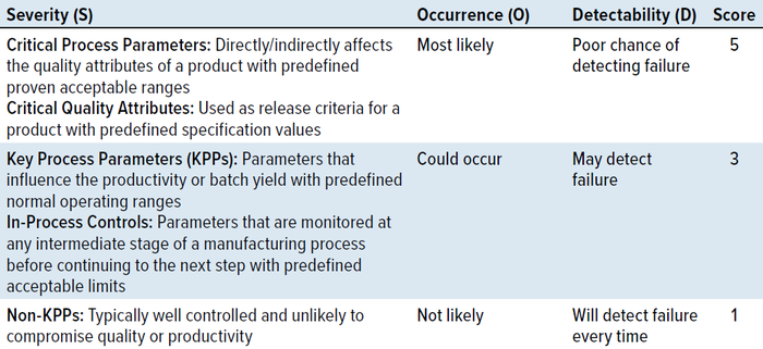
In alignment with the ASTM recommendations, you can design a risk-assessment matrix by scoring the attributes/parameters to be monitored in your PPQ runs based on those three criteria (Table 1). Severity scores are based on the potential impact on product quality or on process productivity and consistency. Occurrence scores are based on controls in place, with the highest score assigned when the rate of occurrence is unknown. Detectability scores are based on the availability and implementation of testing methodologies and monitoring systems. Some test methods, such as those measuring bioburden, carry some level of uncertainty based on sample volume and thus are rated with a medium risk score. Attributes are rated with a low risk score if well-defined test methods with high precision and repeatability are available.

Table 1: Risk-assessment scoring matrix.

Table 2: Guidance for selecting statistical confidence (1 – α) and population proportion to cover (p) using the ISPE method; RPN = risk priority number.

A risk priority number (RPN) is generated from the product of those three scores: RPN = S × O × D. The risk for each parameter is classified as high, medium, or low based on the RPN scoring matrix in Table 2. That table also includes recommendations for setting statistical confidence (1 – α) and residual risk (1 – p) by defining the proportion (p) of a population to cover based on risk classification.

The confidence level (1 – α) and p for different risk categories (Table 3) are adopted from a guidance document from the International Society for Pharmaceutical Engineering (ISPE) (4). Different values for each can be adapted based on published articles, regulatory documents, and/or a company’s own quality risk management policies that are considered to be appropriate for a given manufacturing process.

Sample-Size Reliability of Historic Data Used To Gain Process Knowledge: Often, only limited data are available from stage 1 (process development and characterization phase) before a program enters stage 2. Thus, the first step in calculating the number of PPQ runs is to ensure that the sample size used to gain process knowledge will be reliable. One method of doing so is to assess the power of estimation as a function of sample size used at an acceptable statistical confidence.

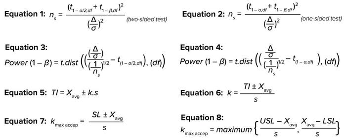
You can calculate the required sample size for a t-test at the desired confidence, power, and detectability with Equation 1 (for a two-sided test) and Equation 2 (for a one-sided test), where n_s is the sample size, df = n_s – 1 represents degrees of freedom, and
t_{(1 – α,df)} represents the inverse of the cumulative t distribution at 1 – α and df (5). Here, the significance value (α) type-1 error often is set at an acceptable value of 0.05, indicating a 5% chance of false rejection for an actually true null hypothesis — or in other words, the statistical confidence (1 – α) is 100% – 5% = 95% (6). For β type-2 errors, the widely acceptable minimum value is 0.20, indicating a 20% chance of failure to reject a null hypothesis that is actually false — or in other words, the statistical reliability (1 – β) is
100% – 20% = 80%.

Equations 1–8.

Detectability/effect (Δ/σ) is the acceptable distance from the mean, expressed as the number of standard deviations, to support a null hypothesis (H₀) that there is no difference between a sample and the population it came from. Therefore, relaxing the criteria for H₀ by increasing the value of δ will decrease the required sample size. A Δ/σ value of 1.0–1.5 has been reported as acceptable for calculating the required sample size (7). The FDA guidance document on “statistical review and evaluation” states that a Δ/σ value of 1.5 at 90% confidence (1 – α) is adequate to conclude equivalence between two groups. For the purposes of this discussion, that value is the size of a sample that can represent the population (8).

Equations 1 and 2 for sample size can be rearranged to solve for the power of estimation, as shown in Equation 3 (for a two-sided interval) and Equation 4 (for a one-sided interval), where t.dist is the cumulative distribution function of the t distribution. According to Cohen in 1988, the generally accepted minimum power (1 – β) is 80% for a confidence
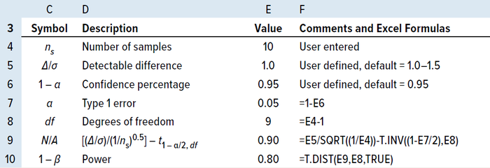
(1 – α) of 95% (6, 9). Table 3 depicts an example of a two-sided interval, with the power calculated for a randomly selected sample size of 10 using MS Excel software.

Table 3: MS Excel power calculation for a sample size of 10.

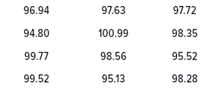
Table 4: Twelve randomly generated data values for illustrating the tolerance interval (TI) method.

Tolerance Interval Method
TI describes the range that gives a fixed proportion (p) of a population at a stated statistical confidence (1 – α), based on the assumption that the sample data are taken from a normally distributed population (5, 7). A two-sided TI is expressed as shown in Equation 5, where TI represents the tolerance interval; X_avg and s represent the sample mean and standard deviation, respectively; and k is the tolerance interval estimator. The latter expresses how many standard deviations away from the mean will cover a certain fixed proportion of a population at the desired statistical confidence.

Equation 5 can be rearranged to become Equation 6. Replacing the TI by a specification limit (SL) will yield the maximum acceptable tolerance estimator (k_{max, accep}), which ensures that a process remains within predefined specifications and can be written as Equation 7. In other words, k_{max, accep} is the maximum acceptable distance in standard deviations from the mean for an acceptable specification (10). It can be elaborated upon as shown in Equation 8 for attributes with two-sided acceptable limits or specification limits.

Uncertainty with Sample Mean and Standard Deviation: Limited sample sizes available before stage 2 process qualification bring uncertainty to using the sample mean and standard deviation. You can compensate for that by replacing the sample mean and standard deviation with their respective confidence intervals. A confidence interval is a range that gives a single-valued parameter, such as the mean or standard deviation, of a population at a stated confidence.

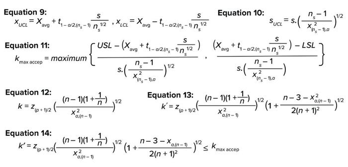
Equations 9 and 10 show confidence intervals around the mean and standard deviation (5). Here, x_UCI and x_LCI represent the upper and lower confidence-interval values for the mean, and S_UCL represents the upper confidence-interval value for the standard deviation. Substituting Equations 9 and 10 in Equation 8 yields the maximum acceptable tolerance estimator (k_{max, accep}) with compensation for uncertainty associated with the small sample size (Equation 11).

Equations 9–14.

In 1969, Howe gave an estimate of the TI estimator k value as a function of sample size (n), confidence (1 – α), and proportion (p), as shown in Equation 12 (5), where z and χ² are the inverse of the cumulative normal distribution and chi-square distribution, respectively. Later, Guenther corrected Howe’s approximation by using k′ instead of k for smaller samples, as shown in Equation 13 (5).

To ensure that a process remains within predefined specification limits, the confidence estimator (k′) should be lower than the maximum confidence limit estimator (k_{max, accep}). Now the number of PPQ runs (n) can be calculated by using Excel software’s solver function or by iteratively changing the value of n starting from n = 3 until the k′ value is approximately ≤(k_{max, accep}), as shown in Equation 14 (7).

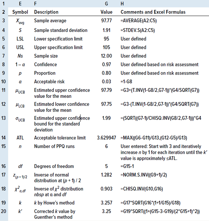
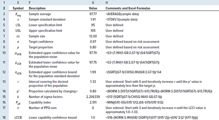
Example for Sample Data and Risk Assessment: For an example of the TI method, I used the Excel function =NORM.INV(RAND(),100,2) to generate 12 random samples following a normal distribution, with a mean of 100 and a standard deviation of 2. I set the upper and lower specification limit values to 95 and 105, respectively.

Assume a case in which the random variable is a critical quality attribute (CQA), but there is no clear understanding of the control strategy, and the test method has high inherent variability. According to the risk- assessment matrix in Table 2, the PRN score for those values is

PRN = 5 (S) × 5 (O) × 3 (D) = 75

therefore, the risk is considered to be high. Hence, the target confidence is set at 0.97, and the proportion is set at 0.80, as determined using Table 3. See Table 5 for the results.

Table 5: Calculating the number of process performance qualitification (PPQ) runs by the TI method in an MS Excel spreadsheet for two-sided specifications.

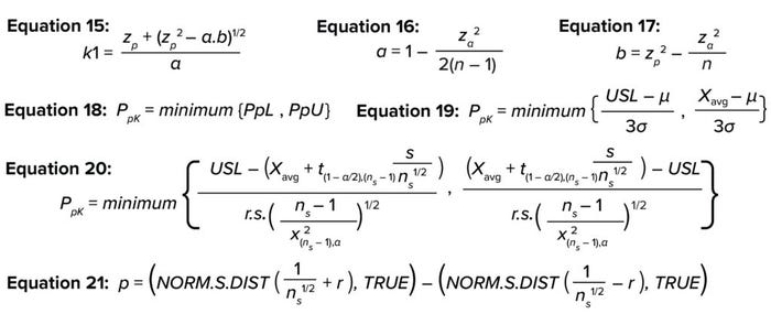
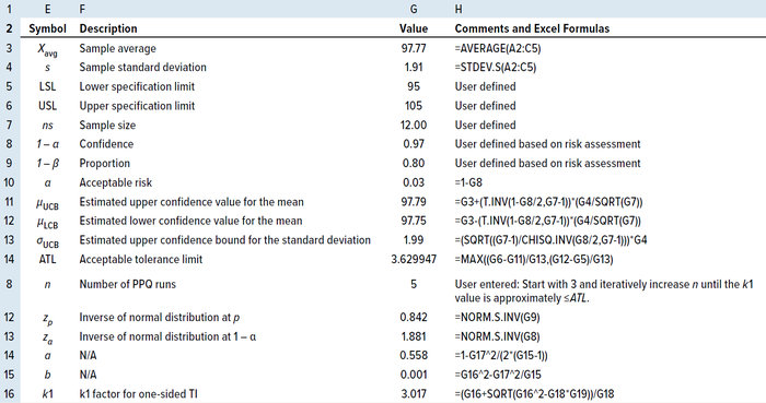
One-Sided TI: For a one-sided TI, Natreilla gives an approximate value for the k factor as in Equation 15 (5), where a is defined as in Equation 16 and b as in Equation 17. Table 6 shows the results of applying the same example data in the two-sided TI method to illustrate the use of the TI method for a one-sided TI, using only the upper specification limit.

Equations 15–21.

Table 6: Calculating the number of PPQ runs by the TI method for a one-sided specification.

Process Capability Method
Process Performance Index: The ability of a process to meet predefined specifications is determined by P_pK’, which is defined as the ratio of the distance from the process mean and nearest specification to the one-sided spread of the process (3σ variation) based on the overall standard deviation for a normally distributed population (11). P_pK is calculated as shown in Equations 18 and 19 (12), where P_pK is the process performance index; P_pL and P_pU are the lower and upper process performance indices, respectively; USL and LSL represent the upper and lower specification limits, respectively; and μ and σ represent the underlying true population mean and overall true population standard deviation, respectively.

Uncertainty with Sample Mean and Standard Deviation, and with Sigma Factor: Equation 19 for P_pK typically is used for sample sizes of at least 25. However, the sample size generated before stage 2 process qualification often is less than 25, and the underlying true population mean and population standard deviation usually are unknown at that stage. As discussed for the TI method above, you can compensate for the uncertainty of using the sample mean and sample standard deviation from a small sample size by replacing them with confidence intervals around the mean and standard deviation.

The sigma factor of ±3 in the 3σ term in Equation 19 represents the number of standard deviations from the mean that covers 99.7% of the true population. However, because the proportion of the population to cover is based on risk assessment, and for accommodating the uncertainty involved in a limited available sample size, the term of ±3 is replaced in Equation 19 with r, which is the number of sigma factors from the mean covering the desired proportion of the population.

By substituting Equations 9 and 10 in Equation 19, you can rewrite P_pK as in Equation 20. The r value can be calculated iteratively by increasing the value of k from k = 0 in Equation 21 to achieve a desired population proportion based on the risk assessment.

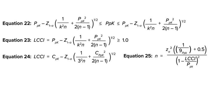
Uncertainty with P_pK Estimation: Equation 22 expresses Bissell’s approximated confidence interval for a capability index that accommodates uncertainty for the P_pK calculation (13–15). The FDA’s 2011 PV guidelines states that current good manufacturing practice (CGMP) regulations require manufacturing processes to be “designed and controlled to assure that in-process materials and the finished product meet predetermined quality requirements and do so consistently and reliably” (1). A capability index value of 1.0–1.3 indicates that a given process is capable of routinely meeting its specifications — and is most likely to meet them regularly (12). That would be in alignment with the expectation from the PV guidance. Therefore, the number of PV batches (n) required can be calculated by iteratively increasing the value of n from 3 to achieve a lower capability confidence interval (LCCI) of 1.0–1.3 in Equation 23.

Equations 22–25.

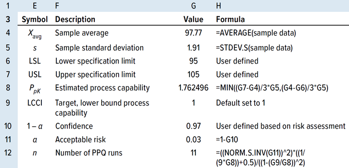
Approximating the Number of PPQ Runs for a Sample Size of ≥30: When the available sample size is ≥30, the LCCI equation can be simplified by replacing k with 3 and rearranging to give Equation 24 (14). Wu and Kuo rearranged and solved for the number of PPQ runs needed to meet a predefined specification at a specified confidence level (α), as shown in Equation 25, when the available sample size was ≥30 (13). Tables 7 and 8 show results from applying the same randomly generated data used for the TI method above to illustrate use of the PpK method.

Table 7: Process capability (PpK) method for calculating the number of PPQ runs using an MS Excel spreadsheet for a sample size of <25.

Table 8: Calculating the number of PPQ runs by the PpK method using an MS Excel spreadsheet for sample sizes >25.

Intrabatch and Interbatch Variations
Both the TI and PpK methods for calculating the number of PPQ runs take interbatch and intrabatch variation into consideration.

Intrabatch Variability: Data gained during stage 1 of a biologic product’s life cycle include results from biomanufacturing process-development runs, process-characterization runs at bench scale, and scale-up runs at both pilot and manufacturing scales. Often those operations introduce sources of variation to the process from differences in raw-material lot numbers, operation scales, controller makes and models, condition ranges, and staff skills and abilities. Therefore, data from stage 1 pre-PPQ studies will provide a reliable measure of variability within batches (16).

Interbatch Variability: Large data sets are required to assess batch-to-batch variability reliably. However, because sample data typically are limited before and after PPQ runs, it will be difficult to make reliable assessments of interbatch variation. Therefore, compensating for the risk of uncertainty that comes with limited sample sizes by using the confidence and tolerance intervals (as above) when calculating the number of PPQ runs will incorporate interbatch variability.

Especially Applicable for Advanced Therapies
Process and product understanding are established using data from early process development, from previous experience with similar process, from scale-up activities, and from scale-down–model verification runs and process-characterization studies (15). In-depth product knowledge for defining CQAs and characterizing critical process parameters (CPPs) of biomanufacturing processes with detailed understanding of variability introduced from raw materials and process operations are yet to be established for new therapeutic technologies such as ex-vivo gene-modified cell-based therapies and in vitro gene therapies (17).

For therapeutic proteins, three batches traditionally have been considered to be sufficient for process qualification. A certain amount of risk is associated with low product knowledge for new technologies needing to meet robust acceptable ranges. Based on available product knowledge, a risk-based approach to meeting predefined specifications at a predefined statistical confidence can be used to calculate the adequate number of PPQ runs, as recommended in the 2011 FDA validation guidance document (1).

Above I have provided detailed, step-by-step guidance for two such methods based on process capability and process tolerance, including illustrative examples based in Excel spreadsheets for easy adaptation and implementation by readers. A single statistical method cannot fit all biomanufacturing processes — or even all attributes assessed for a single process. Thus, when selecting statistical methods and performing risk assessments to set confidence values, companies should evaluate carefully not only the nature of their data and the reliability of available historical knowledge, but also the costs associated with manufacturing, testing, and releasing a given product.

References
1 CBER/CDER/CVM. Guidance for Industry: Process Validation — General Principles and Practices. US Food and Drug Administration: Rockville, MD, January 2011; http://www.fda.gov/downloads/Drugs/Guidances/UCM070336.pdf.

2 James D, et al. Stage 2 Process Validation: Regulatory Expectations and Approaches To Determine and Justify the Number of PPQ Batches. BioPharm Int. 30(7) 2017: 52–58; https://www.biopharminternational.com/view/stage-2-process-validation-regulatory-expectations-and-approaches-determine-and-justify-number-ppq-0.

3 ASTM E2476-22. Standard Guide for Risk Assessment and Risk Control as it Impacts the Design, Development, and Operation of PAT Processes for Pharmaceutical Manufacture. American Society for Testing and Materials: West Conshohocken, PA, 17 November 2016; https://www.astm.org/e2476-22.html.

4 Bryder M, et al. Topic 1: Stage 2 Process Validation — Determining and Justifying the Number of Process Performance Qualification Batches (Version 2). International Society for Pharmaceutical Engineering: Bethesda, MD, 1 February 2014; https://ispe.org/publications/papers/stage-2-process-validation-process-performance-qualification-batches.

5 NIST/SEMATECH. Engineering Statistics Handbook. National Institute of Standards and Technology: Gaithersburg, MD, 2012; https://doi.org/10.18434/M32189

6 Lakens D. Calculating and Reporting Effect Sizes to Facilitate Cumulative Science: A Practical Primer for T-Tests and ANOVAs. Front. Psychol. 4, 26 November 2013; https://doi.org/10.3389/fpsyg.2013.00863.

7 Durivage M. How To Establish Sample Sizes for Process Validation Using Statistical Tolerance Intervals. Bioprocess Online 27 October 2016; https://www.bioprocessonline.com/doc/how-to-establish-sample-sizes-for-process-validation-using-statistical-tolerance-intervals-0001.

8 Weng Y. Statistical Review and Evaluation. US Food and Drug Administration: Rockville, MD, 21 March 2016; https://www.fda.gov/media/105013/download.

9 Schuirmann DJ. A Comparison of the Two One-Sided Tests Procedure and the Power Approach for Assessing the Equivalence of Average Bioavailability. J. Pharmacokin. Biopharmaceut. 15(6) 1987: 657–680; https://doi.org/10.1007/bf01068419.

10 Vasta A. Determining Sample Size for Specification Limits Verification with Tolerance Intervals. Qual. Reliabil. Eng. Int. 37(5) 2021: 1718–1739; https://doi.org/10.1002/qre.2821.

11 Cohen J. Statistical Power Analysis for the Behavioral Sciences (Second Edition). Lawrence Erlbaum Associates: Hillsdale, NJ, 1988.

12 TR 59. Utilization of Statistical Methods for Production Monitoring. Parenteral Drug Association: Bethesda, MD, November 2012; https://www.pda.org/bookstore/product-detail/1842-tr-59-utilization-of-statistical-methods.

13 Charoo NA. Estimating Number of PPQ Batches: Various Approaches. J. Pharmaceut. Innov. 13(2) 2018: 188–196; https://doi.org/10.1007/s12247-018-9316-2.

14 Wu CC, Kuo HL. Sample Size Determination for the Estimate of Process Capability Indices. Info. Management Sci. 15(1) 2004: 1–12.

15 Yang H. Emerging Non-Clinical Biostatistics in Biopharmaceutical Development and Manufacturing. CRC Press: New York, NY, 2016.

16 Pazhayattil A, et al. Stage 2 Process Performance Qualification (PPQ): A Scientific Approach To Determine the Number of PPQ Batches. AAPS PharmSciTech 17(4) 2015: 829–833; https://doi.org/10.1208/s12249-015-0409-7.

17 Heidaran M. Manufacturing Controls at Commercial Scale: A Major Hurdle for the Cell and Gene Therapy Industry. Regulatory Focus 25 April 2019; https://www.raps.org/news-and-articles/news-articles/2019/4/establishing-manufacturing-controls-a-hurdle-for.

Formerly with Novartis Gene Therapies, Naveenganesh Muralidharan is now a senior manager in manufacturing science and technology (MSAT) for AGC Biologics, 5550 Airport Boulevard, Boulder, CO 80301; 1-314-496-8483; [email protected]; www.agcbio.com.