Statistical Properties of WECO Rule Combinations Through Simulations

ADOBE STOCK (WWW.STOCK.ADOBE.COM)

The practice of quality control is promoted by the US Food and Drug Administration (FDA) and European Medicines Agency (EMA). A number of process control charts are used in many biopharmaceutical companies to increase production and lower process costs. Here we focus on performance of three commonly used control charts: Shewhart control charts with WECO and supplementary rules, monitoring charts with exponentially weighted moving average (EWMA), and cumulative sum (CUSUM) charts.

WECO rules got the name from a quality control handbook published by the Western Electric Company in 1956 (1). Those rules and the additional four supplementary rules are used with Shewhart control charts in statistical process control (SPC) for detecting out-of-control signals before control limits are exceeded. For simplicity, we refer to all eight rules as WECO rules. In the handbook, the authors extensively discuss the range
of tests to detect abnormal patterns. The theoretical probability of violating each single rule when a process is in control (false-positive detection) has been investigated thoroughly (2–4). However, few studies have discussed combinations of certain WECO rules (5, 6). The first time (T) at which a process experiences its first out-of-control signal is called running length (RL), and the distribution of T is called the running length distribution. The mean of that distribution — the average running length (ARL) — is used frequently as a measure in SPC for evaluating and comparing performances of different methods.

Equations

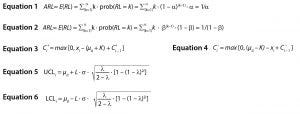
Under an in-control (stable) process (H₀ is true, where H₀ is the assumption that the current process is in conrol or stable), the chance to observe an out-of-control (OOC) signal is defined as α = prob(a Shewhart chart signals on a given sample | H₀ is true), and ARL can be calculated by Equation 1. Here, E(.) is the expectation of the random variable in parenthesis. For an out-of-control ARL, the actual process is OOC (H₁ is true, where H₁ is the assumption that the current process is out of control or unstable), the chance to observe a true OOC signal is 1 – β = prob(a Shewhart chart signals on a given sample | H₁ is true). Similarly, the OOC ARL can be calculated by Equation 2.

For common 3σ control limits, α = 0.0027, so ARL ≈ 370, which suggests that it takes 370 samples on average before a chart sets off a false alarm. In our simulation settings, we use ARL = 370 as a standard to adjust the parameters for CUSUM and EWMA methods for in-control process. In practice, we’d like the in-control ARL to be as large as possible and OOC ARL to be as small as possible.

A CUSUM chart is one of the most popular types of control charts. It was proposed initially by E.S Page for monitoring change detection (7). Unlike Shewhart control charts, CUSUM charts use the information from previous observations by displaying the cumulative sum of a deviation of sample values from a specified target. Therefore, CUSUM charts are more efficient than Shewhart control charts for detecting small process changes, whereas Shewhart charts are superior for detecting large mean shifts. The particular version of CUSUM used herein is the Tabular CUSUM, written in Equations 3 and 4. Here, K is the reference value (or allowance value) and is often chosen about halfway between a target value and an OOC value mean. The process is out of control if either C_i⁺ or C_i^– exceeds the decision interval H. In this discussion, K = 0.5 and H = 4.77 are used to match in-control ARL = 370 of the Shewhart control chart.

One challenge to applying the CUSUM method for scientists is properly choosing values for parameters K and H. Without knowing the OOC process mean, which is commonly unknown, it can be very difficult to choose K and H beforehand. The impact of K and H on ARL is complicated. Empirical methods through computational procedures to evaluate an ARL for given combinations of K and H are available in literature (1). Proper choice of selecting K and H for an unknown process, however, is a challenge.

EWMA first was introduced by Roberts (8). Similar to the CUSUM method, EWMA uses information from previous data points, so it’s a good choice for detecting small changes in a process (1) by adding weights to previous data. The test statistic is defined as z_i = λ ⋅ x_i + (1 – λ) ⋅ z_{i – 1}, where 0< λ ≤1 is a constant and the starting point z₀ = μ₀. Here μ₀ could be the process target or the average of historical data if a process target is unknown and x_i is the ith sample observed.

Equations 5 and 6 describe upper and lower control limits. A violation is detected when z_i is out of the control limits UCL_i or LCL_i. Herein we use L = 2.86 and λ = 0.2 to match in-control ARL = 370 of Shewhart control chart.

Similarly, it is a challenge to choose the two parameters: λ and L for the EWMA method. The parameter λ controls how much “memory” the chart has. The smaller λ is, the better will be detection of small changes. The larger λ is, the better detecting of large changes. For different λ, L can vary as well. The EWMA ARL estimation relies on combinations of λ and L.

Unlike CUSUM and EWMA methods, Shewhart control charts with WECO rules are simple and straightforward to implement. No parameters need to be chosen for any of the rules. Eight commonly adopted abnormal patterns (corresponding to eight WECO rules) are widely implemented in several software programs (e.g., SAS, Minitab, R, and JMP). Those eight WECO rules used with control charts can enhance greatly the sensitivity of Shewhart chart to different changes in a process. A good practice is to apply WECO rules to monitor product quality and detect deviations from a stable process early. Using all eight WECO rules together is impractical. Some ad hoc rule combinations usually are selected.

Intuitively, combining different WECO rules increases sensitivity of detection, but it also increases the probability of making false alarms when a process is in control. Statistical properties of single rules and limited combinations for several rules are well studied (3, 4), but the statistical properties of WECO rule combinations have not been studied thoroughly.

To circumvent the theoretical derivation, we alternatively adopt here the Monte Carlo simulation methods to evaluate ARL for in-control (stable) and OOC processes, both with independent and correlated data. Such evaluation fills in the blank and paves the way for practitioners who already have experiences in using WECO rules but are not sure about what rules should be used together in their respective applications.

WECO Rules and Shewhart Control Chart
Western Electric Company Rules (WECO): The following are the eight WECO rules as used in Minitab software.

Rule 1: One data point is greater than three standard deviations (SDs) from the center line. (This rule is to identify a single data point that is out of the acceptable range.)

Rule 2: Nine data points are in a row on the same side of the center line. (The ideal stable process is assumed to be up and down around the center line. A large block of data points on the same side of the center line indicates that a process mean is shifted.)

Rule 3: Six data points are in a row, all increasing or decreasing. (This rule is an indicator of possible mean shift.)

Rule 4: Sixteen data points are in a row, alternating up and down. (When data points routinely alternate up and down, it shows a high negative correlation between neighboring observations, which is abnormal for a stable process. For an in-controlprocess, it is not expected to observe correlation between neighboring data points.)

Rule 5: Two out of three data points on the same side are greater than two SDs from the center line. (For a normally distributed in-control-process, about 95% of data points should be within two SDs. The chance of violating this rule is 0.00306. This rule is used to detect increase in process variation.)

Rule 6: Four out of five data points on the same side are greater than one SD from the center line. (For a normally distributed in-control-process, about 62% of data points should be within 1 SD. This chance to violate this rule is 0.00553. This rule is also used to detect increase in process variation.)

Rule 7: Fifteen data points are in a row within one standard deviation of the center line. (Too many data points within one SD indicates a decrease in process variation.)

Rule 8: Eight data points in a row are greater than one SD of the center line. (This is another rule to detect increase in process variance.)

A normal pattern is one in which the observed points fluctuate randomly up-and-down from the process mean. A stable (or in control) process produces mostly a normal pattern. Other types of the patterns are classified as abnormal. Abnormal patterns and OOC are used interchangeably herein.

Shewhart Control Chart: The control chart invented by Walter A. Shewhart in the 1920s is a tool for analyzing process variability over time (1). It is a graphical depiction of process variability with either normal or abnormal patterns. A control chart’s central line represents the average values in a series of monitored samples over its monitoring time. And the two-sided or one-sided control limit is set up around the center line so that when a process is normal (stable), nearly all points in the chart fall between the control limits. For example, ±3σ controls limits are used widely with control charts such that about 99.7% of process data fall within the control limits for a stable process. If some points are outside the control limits (abnormal process is indicated), a follow-up corrective action or some improvement can be initiated. The effect of WECO Rule 1 can be thought of as the same as that of a Shewhart control chart.

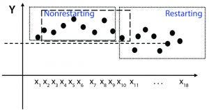
Figure 1: Control process with and without restarting

Monte Carlo Simulation
ARL is used commonly to evaluate the performance of different methods. Running length is the number of data points that the first-rule violation is identified. For an in-control process, ARL reflects the mean of false alarm times and therefore is preferred to be longer (larger). But for an out-of-control process, ARL reflects the mean delay of true alarm times and thus is preferred to be shorter (smaller).

However, we have noticed that ARL can be defined differently depending on whether a process gets restarted after an OOC signal is detected. Taking the second WECO rule as an example, suppose the nine points in sequence (x_i …, x_{i + 8}) are on the same side of center line, and the second WECO rule is violated. The restarting process starts a scan from x₁₀, and a nonrestarting process starts from x₂ (Figure 1). The probability that the next sequence of nine data points (x_i + 1 …, x_{i + 9}) violates the second rule again is 0.5/(2 × 0.5⁹) = 128 times higher than a sequence of all nine new data points. The ARL would be significantly longer if simulation is restarted compared with what it would be if the simulation moves on after an OOC signal is detected.

Table 1: Running length distribution of eight WECO rules without restart

Theoretical ARL for each of the eight WECO rules has been derived through an enumeration method (2, 9). In the derivation, the sequence is assumed to be infinitely long, and it is not restarted when a violation is observed. In the first proof-of-concept Monte Carlo simulation, a sequence with one billion data points is generated, and all violations are recoded. Table 1 shows the running length distribution results of each single WECO rule’s theoretical derivation and the results through simulation. The percentiles at 0%, 25%, 50%, 75%, and 100% of running length are adopted as quantitative measurements of the distribution of that variable. The simulation and the theoretical results agree well, and the differences all are within 0.5%.

Table 2: Running length distribution of eight WECO rules with restart

However, if the sequence is restarted after a violation is observed, running length distributions all become longer except for Rule 1. Because each single data point is independent and identically distributed (IID) for a stable process, and Rule 1 involves only a single data point, then it makes no difference whether the process is restarted. Table 2 shows the running length distributions (the five percentiles of the distribution) of each single WECO rule when the sequence restarts after a violation is observed.

In practice, manufacturing will be halted, and an investigation of a production process will be initiated when a violation is detected. A process is restarted when the root cause is identified and removed. Thus, evaluation of the running length of the first violation (RLFV) is more important. For that reason, we adopt a simulation strategy that reflects this consideration. The following is the simulation strategy we adopted here.

Step 1: Generate a data sequence with 500 data points from a first-order autoregressive model: x_i = μ + φx_i – 1 + ε, where ε ~IID N(0, σ²) and –1< φ <1. When φ = 0, the model is reduced to a simple IID normal distribution. The value for μ is the process mean, and μ = 0 for a stable process.

Step 2: Run WECO rules and record the first position in the sequence when a violation is identified.

Step 3: If no violation is identified, repeat step 1 to generate another 500 data points and append them to the previous sequence.

Step 4: Repeat steps 2 and 3 until a violation is identified. If no violation is identified in one million data points, then record “NA,” and restart the simulation.

This simulation procedure is used in all simulation studies, including single WECO rules, combination of WECO rules, EWMA, and CUSUM. The parameters in EWMA and CUSUM are selected to match in-control ARL = 370 of a Shewhart control chart. And in all simulations, L = 2.86 and λ = 0.2 are used for EWMA method and K = 0.5 and H = 4.77 for CUSUM method. Different disturbances are introduced into the normal process (Gaussian distribution) by adding a constant mean shift (μ), increased variability (σ), or different autocorrelation (φ) to the data. Both process mean shift and variability change are standardized to the multiples of the SD. Process mean shift μ varies as 0, 0.5, or 3 SD, and variability σ changes as 1, 2, or 3 SD. Positive autocorrelation coefficient φ changes among 0, 0.25, 0.5, or 0.95. In total, there are 36 different simulation settings.

Simulation Results
The eight WECO rules can be combined in many ways. For simplicity in this evaluation, we investigate only the performance of a combination of two WECO rules by comparions with EWMA or CUSUM. Running length distributions for more than two rule combinations can be generated through our R package “weco” (https://cran.r-project.org/web/packages/weco/index.html), or you can request the code from us.

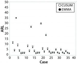
Figure 2: ARLs between CUSUM and EWMA under 36 different scenarios; two ARLs greater than 50 are not included in the graphs.

We have discovered that an EWMA chart has slightly smaller ARLs in most cases (46 out of 48) than CUSUM. Therefore, EWMA has a subtle advantage in general over CUSUM in detecting an out-of-trend signal of a positively autocorrelated process using parameters we specified. Han and Tsung reached the same conclusion (10). Figure 2 shows detailed ARLs in different simulation settings between EWMA and CUSUM. For convenience — and considering that most differences of ARLs between EWMA and CUSUM are no more than 1 (additional table presented online only at bioprocessintl.com) — we report only the results of WECO rule combinations compared with the CUSUM method.

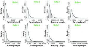
Figure 3: Empirical run-length distribution of eight single WECO rules

Single WECO Rule Compared with CUSUM/EWMA: The running-length distribution is highly skewed for all WECO rules (Figure 3). ARL is used to evaluate the performance of various control chart methods.

Figure 4 shows the logarithm of ARLs among eight single WECO rules and the CUSUM method. For a stable process (μ = 0, σ = 1, φ = 0), most rules perform better than CUSUM except Rule 6 because it has shorter ARLs than the CUSUM method (larger false positive rate).

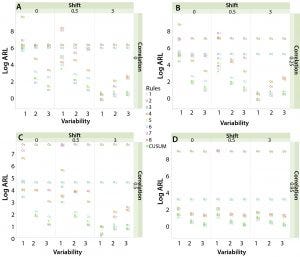
Figure 4: Single rule and CUSUM; log (ARL) when (A) autocorrelation = 0; (B) autocorrelation = 0.25; (C) autocorrelation = 0.5; (D) autocorrelation = 0.95

Rules 3 and 4 are not sensitive to mean shift, variability change, or autocorrelation because their ARLs are above CUSUM results when a disturbance presents. A similar conclusion can be made for Rules 2 and 8, except in cases in which μ = 0 and σ = 1 regardless of autocorrelation.

Rules 5 and 6 perform similarly, although Rule 5 is slightly more sensitive. Rule 1 is without doubt the most useful WECO rule in control charts because its ARL values are below CUSUM results most of the time in presence of disturbances.

WECO Rule 7 is insensitive to autocorrelation, and it is not applicable after moderate mean shift and variability increases more than 1 SD.

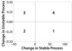
Figure 5: Discrete sensitivity and specificity

Combination of WECO Rules Compared with CUSUM/EWMA: When it comes to the discussion of combining WECO rules, the interesting questions are the following: What will be the performance when those rules are combined compared with the CUSUM method? Are Rule 1 and Rule 5 still the favorites while keeping reasonable false-positive rates?

Combining rules will increase false-alarm rates. So selecting necessary combinations of WECO rules to balance sensitivity (true positive rate) and specificity (true negative rate) is always preferred. Thirty-five discrete sensitivity and specificity plots are generated. The plots are discrete because they show the performance of only limited combinations of WECO rules. Those plots represent performance of combination rules relative to the benchmark CUSUM method under 35 different disturbance cases. The x-axis is the change in process stability, which is defined as the change in stable process = (ARL_weco – ARL_cusum) / ARL_cusum × 100%.

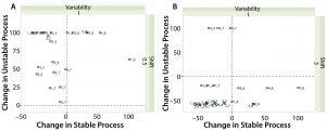
Figure 6: (A) Discrete sensitivity and specificity plot when autocorrelation φ = 0, variability σ = 1, and mean shift μ = 0.5; (B) discrete sensitivity and specificity like plot when autocorrelation φ =0 , variability σ = 1, and mean shift μ = 3

Similarly, we can define the change in an unstable process. For each combination rule, there are 35 different change in unstable process values. Absolute changes greater than 100% are forced to be 100% for demonstration purposes. As we discussed above, in a stable process, the longer the ARL, the better performance of the method. So if the change in a stable process is >0, then a pair of WECO combinations outperforms the benchmark method. For an unstable process, the smaller the ARL, the more sensitive a method will be. Hence, the change in an unstable process is <0 when it beats the benchmark method. We divide the change plot in four regions (Figure 5). The combination rules that fall into region 1 are those with both good sensitivity and specificity. Region 2 are those with good sensitivity only. Region 4 are those with good specificity only. The 35 plots are included in the online version of this article. Because of the space limitations of print, we display only a few of them in Figures 5–8.

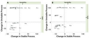
Figure 7: Discrete sensitivity and specificity like plot when (A) autocorrelation φ = 0, variability σ = 2, and mean shift μ = 0; (B) when autocorrelation φ = 0.95, variability σ = 3, and mean shift μ = 0

Figure 6 shows that as a process scales up while conditions are kept the same, most pairs of combination rules demonstrate a sensitivity advantage over the CUSUM method, whereas the CUSUM method dominates in small mean-shift cases. However, when process variability increases or when autocorrelation is introduced into a system, the CUSUM method no longer has advantage for a small mean shift (Figure 7).

While searching for a pair of rules that fall into region 1 (demonstrating both good sensitivity and specificity), we find that two pairs appear substantially more frequently than others. Rule 5 with Rule 8 appears 29 out of 35 times, and Rule 1 with Rule 8 shows up 26 out of 35 times in region 1. The only cases in which both pairs do not perform well (not in region 1) are when there is no process variability change (σ = 1) and a small mean shift (μ = 0 or μ = 0.5) under small-to-moderate autocorrelation (φ ≤ 0.5).

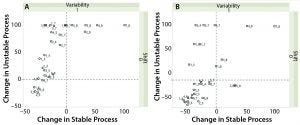
Figure 8: Discrete sensitivity and specificity like plot when (A) autocorrelation φ = 0.25, variability σ = 1, and mean shift μ = 0.5; (B) autocorrelation φ = 0.95, variability σ = 1, and mean shift μ = 0

As autocorrelation increases, more WECO rule combinations show better sensitivity than CUSUM, even when variability and mean shift change are small (Figure 8). More pairs of WECO rules appear in region 1 and 2 as autocorrelation (φ) increases. Thus, a Shewhart control chart with a combination of WECO rules performs well in the presence of high autocorrelation.

The traditionally known advantage of CUSUM/EWMA over Shewhart control charts in detecting small mean shifts (1, 11) no longer holds when there are variability changes and autocorrelations. Simulation results showed that pairs of WECO Rules 1 and 8 and Rules 5 and 8 are more sensitive than other paired rules in detecting an OOC condition, regardless of a number of disturbances. However, if a process is expecting a small disturbance (either a small mean shift, small variability change, or small autocorrelation), the CUSUM and EWMA methods using default parameters are still preferred.

The Right Combination
Shewhart control charts are among the most important and useful techniques in statistical process control. Their capabilities are enhanced greatly when coupled with WECO rules. Applying several WECO rules simultaneously is more powerful for detecting abnormal patterns. When WECO rule combinations are applied, the running length is shortened considerably, making them more powerful or more sensitive for detecting an OOC signal. However, imposing more rules at the same time not only makes application more complicated, but also raises the false alarm rate. Selecting a necessary combination of WECO rules to balance the sensitivity, and specificity rate is always a challenge.

We have conducted comprehensive simulation studies that mimic the situations with changing process variability, mean shift, and autocorrelation. RL distributions of WECO rule combinations were investigated by comparing them with those of benchmark methods CUSUM and EWMA. The simulations show that single Rules 1 and 5 are more beneficial than other rules in different abnormal circumstances. Combinations of Rules 1 and 8 and Rules 5 and 8 are favorable in most situations. The simulation studies shown here provide the first practical guidance for choosing WECO rule combinations.

We have developed a statistical package to facilitate investigations of WECO rule combinations. The package includes implementation of all eight WECO rules. It allows users to make combinations of them to investigate the performance under user-specified conditions. The package name is “weco” and can be downloaded for free from the CRAN website (https://cran.r-project.org/web/packages/weco/index.html).

Acknowledgment
The authors thank scientist Hyun Kim and others for raising this topic.

Conflict of Interest Declaration
The authors declare that they have neither financial nor nonfinancial competing interests related to this paper.

References
1 Montgomery DC. Introduction to Statistical Quality Control, 6th ed. Wiley: New York, NY, 2013.

2 Champ CW, Woodall WH. Exact Results for Shewhart Control Charts with Supplementary Run Rules. Technometrics 29(4) 1987: 393–399.

3 Walker E, Philpot JW, Clement J. False Signal Rates for the Shewhart Control Chart with Supplementary Runs Tests. J. Qual. Technol. 23 (3) 1991: 247–252.

4 Griffiths D, et al. The Probability of an Out of Control Signal from Nelson’s Supplementary Zig-Zag Test. Centre for Statistical and Survey Methodology, University of Wollongong, Australia, 2010; http://works. bepress.com/dgriffiths/5.

5 Trip A, Does R. Quality Quandaries: Interpretation of Signals from Runs Rules in Shewhart Control Charts. Qual. Eng. 22(4) 2010: 351–357.

6 Noskievičová D. Complex Control Chart Interpretation. Int. J. Eng. Bus. Manag. 5, 2013: 1–7.

7 Page ES. Continuous Inspection Schemes. Biometrika 41(1) 1954: 100–115.

8 Roberts SW. Control Chart Tests Based on Geometric Moving Averages. Technometrics 1(3) 1959: 239–250.

9 Shmueli G, Cohen A. Run-Length Distribution for Control Charts with Runs and Scans Rules. Communications in Statistics, Theory and Methods 32(2) 2003: 475–495.

10 Han D, Tsung F. Run Length Properties of the CUSUM and EWMA Schemes for a Stationary Linear Process. Statistica Sinica 19(2) 2009: 473–490.

11 Schmid W. On the Run Length of a Shewhart Chart for Correlated Data. Stat Papers 36(1) 1995: 111. doi:10.1007/BF02926025.

Lingmin Zeng is senior principal statistician, Wei Zhao is associate director, Harry Yang is senior director, all at the statistical sciences division at MedImmune LLC, Gaithersburg, MD 20878. Chenguang Wang is assistant professor, and Zheyu Wang is an assistant professor, both at the division of biostatistics and bioinformatics at Johns Hopkins University.

The online version of this article includes an additional data table and 35 additional combination graphs.

Lingmin Zeng, Wei Zhao, Chenguang Wang, Zheyu Wang, and Harry Yang