Multivariate Data-Driven Modeling for Continued Process Verification

Figure 1: A biologics manufacturing process consists of three main steps.

Continued process verification (CPV) is an integral part of process validation for the manufacture of human and animal drugs and biological products (1). It is designed to meet three primary goals: maintain a validated state of products, their processes, and related systems; enable continuous process improvements; and meet regulatory requirements for life-cycle validation.

A CPV program for a biologic product entails regular collection of data related to critical process parameters (CPPs) and critical quality attributes (CQAs) and the preprocessing, analysis, and evaluation of those data to ensure that a biomanufacturing process is in a state of control. Typically, CPV is performed at a univariate level in which each parameter or attribute associated with a process or unit operation is evaluated independently. That creates multiple univariate plots for review. In addition, it results in a loss of information related to the correlation of process parameters and quality attributes. Therefore, generating, assessing, and reporting CPPs and CQAs at a univariate level can be labor intensive and time consuming.

Multivariate data analysis (MVDA) consists of advanced statistical techniques for analyzing large, complex, and heterogeneous data sets. MVDA with its associated metrics can reduce the amount of effort required to monitor multiple CPPs and CQAs and report those findings (with high sensitivity for process deviations). MVDA models can monitor multiple process variables with only few multivariate diagnostics while leveraging useful process information in the correlation structure among CPPs and CQAs. Different industrial applications of MVDA have facilitated process understanding, monitoring, and root-cause analyses (2–5). Regulatory agencies also encourage the adoption of multivariate methods as an effective way to monitor manufacturing processes and product quality (1, 6–8).

Multivariate methods can streamline process monitoring operations and provide the same insights as those gained from performing univariate analyses. Thus, these methods can help biopharmaceutical companies reduce their resource needs for CPV report generation and review.

Below, we demonstrate the implementation of an MVDA CPV approach in biomanufacturing. We present a case study for final product manufacturing (FPM) of a therapeutic protein and the key steps in MVDA model development.

Figure 2: A final product manufacturing process consists of six major steps.

Materials and Methods
Process Overview: FPM is the last biomanufacturing step, following cell culture and purification (Figure 1) in which a drug substance (DS) is obtained from cell culture and purified to achieve a target concentration and formulation. A typical FPM process consists of bulking premade DS, processing that through sterile filters, and filling DS material at desired concentration into vials. Lyophilization transforms the solution into a solid drug product (DP) that can be reconstituted. Finally, containers are capped (Figure 2).

Data Source and Type: A CPV program’s requirements define the scope of a data set (parameters for analysis). Parameters are selected from DP quality attributes and FPM process parameters. Data are obtained from a Biovia Discoverant database (from 3DS), and data types are defined as discrete, continuous, or replicate (9).

Discrete data contain only a single measurements of a material or process (e.g., excipient concentration for each batch of DP manufactured).

Continuous data contain a set of measurements taken over time on the same material or process (e.g., filling weights during a sterile fill process for a DP batch).

Replicate data contain multiple measurements of the same type taken on a material or process (e.g., weights of DS batches used to make a single DP batch).

Software: We used the following to develop and implement multivariate, data-driven models for FPM: KNIME analytics platform 3.6.1 (from KNIME), Simca 15 software (from Sartorius Stedim Biotech), and Python 2.7 software (from Python Software Foundation).

Figure 3: For a cross-validation protocol, a data set is partitioned into training and testing subsets. Models are developed for each of the cross-validation rounds (with different partitioning of a data set). Cross-validation outcomes from all models are averaged to estimate a model’s final predictive ability.

MVDA statistical techniques and algorithms are used to analyze data from more than two variables jointly. Such algorithms can be used to detect patterns and relationships in data. Applications include clustering (detecting groupings), classification (determining group and class memberships), and regression (determining relationships among inputs and outputs). Algorithms are said to “learn” from those data because of their ability to find patterns from the data they are exposed to without being explicitly programmed with expected relationships. “Unsupervised” learning algorithms are used to obtain an overview of underlying data without a priori information labeling or mapping to a target or output value. Such algorithms can find structure or patterns in data.

Principal Component Analysis (PCA) is an MVDA method for obtaining an overview of underlying data without a priori information and labeling or mapping them to a target or output value (10). PCA can find structure and patterns in data by reducing the dimensionality of data sets in which collinear relationships are present.

The working principle of PCA is to summarize original data by defining new, orthogonal, latent variables called principal components (PCs). Those consist of linear combinations of original variables in a data set. PCs are chosen such that the variance explained by a fixed number of PCs is maximized. Values of original data in a new latent variable space are called scores. Given a dataset described by an n × m matrix X with n observations and m variables, T denotes an n × k matrix containing the k PC values (scores). The coefficients p_jq with j = 1, . . . m and q = 1, . . . k that determine the contribution of each individual variable x_ij with i = 1, . . . n to the principal component are called loadings. The m × k matrix P is called loading matrix, and the relationship between T, X, and P is given in matrix notation by equation X = TPT + E, in which E denotes the n × m residual matrix. The residual matrix contains the variance not explained by the principal components 1 to k. Basilevsky provides and in-depth introduction to PCA (10).

Model quality is assessed with cross-validation and external data sets, if available. To that end, the R² and Q² statistics are evaluated. The R² statistic describes the fraction of the sum of squares explained by a model, and the Q² statistic conveys information about the predictive ability of a model. Eriksson et al. provide a detailed derivation of both (11).

Cross-validation is a model-testing technique to assess whether underlying statistical relationships in data are general enough to predict a data set that was not used for model training. For such techniques, a given data set is partitioned into training and testing subsets. A model is developed using the training data set and then evaluated against the testing subset. Several rounds of cross-validation are carried out (with different partitioning), leading to multiple parallel models (Figure 3). The outcome from all parallel models is averaged to estimate the final predictive power of the final model. The main purpose of cross-validation is to reduce the chance of overfitting, a condition in which a model fits the training data set well but is not general enough to fit an independent data set reasonably well. We performed seven rounds of cross-validation for model testing, and we used cross-validation to determine model complexity (number of components).

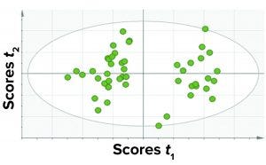
Figure 4: A score plot for PCA model was trained with data for all fill volumes taken together.

Results and Discussion
As we discussed above, our primary focus was to demonstrate the development and application of a multivariate-modeling approach as an alternative to the traditional univariate approach for CPV. Data analysis in this case was performed using a multivariate model developed for FPM. To ensure that the model used for analysis is well suited for satisfying the requirements of multivariate CPV, we adopted an iterative approach for model development. That approach consisted of model selection, training, and testing. Our objective was to evaluate parameters related to FPM of a therapeutic protein holistically and represent a comprehensive performance of different DP batches. To that end, we proposed the adoption of two multivariate diagnostic metrics to identify excursing batches (rather than using more than 30 univariate plots corresponding to each parameter).

The multivariate data-driven model developed for an FPM process was based on PCA. All data used for modeling came from batch processes (one data point for a particular parameter per batch) obtained from the Discoverant software. Determination of the best model for FPM CPV is a complex task because it entails evaluating a landscape that is interlaced with multiple dose strengths and different types of parameters. For example, final containers that are filled with different volumes of DP during the FPM process consist of different dosage strengths.

Initially, model evaluation is performed by considering only DP CQAs. In that case during model development process, CQAs are divided into categories — such as protein-related (e.g., purity), molecular-weight distribution, and so on. Those define the attributes of the therapeutic protein itself and process-related CQAs (e.g., excipient concentration and osmolality) that are properties of an excipient in the final container.
To address the complexity of different fill volumes and parameter types, we evaluated several modeling approaches to determine the one that satisfied the requirements of CPV. We organized the modeling activities into three categories: model selection, model training, and model testing.

Model Selection: Evaluation of different modeling approaches is based on quantifying model performance in a way that would help us determine how much information would be captured by the models. For our study, we compared the values of R2 and Q2 for the different modeling approaches and selected the model with the highest values for both metrics. Another criterion for model selection was to find the best combination of parameters and fill volumes that could represent the process in fewer plots. That helped us determine whether it makes sense to have different fill volumes and parameter types in different plots or consider everything together in a single plot. A single plot would mean a single model, whereas multiple plots would mean multiple models for the same information.

We evaluated three modeling strategies:

Among those three, the first approach yielded the best results in terms of the criteria discussed above. Thus, we considered a single PCA model comprising all CQAs (protein- and process-related), all fill volumes, and select CPPs. Because this model contained all parameters and the different fill volumes together, it has a simple structure and is easy to implement and observe results. Figure 4 shows a PCA score plot with multivariate observations (DP batches).

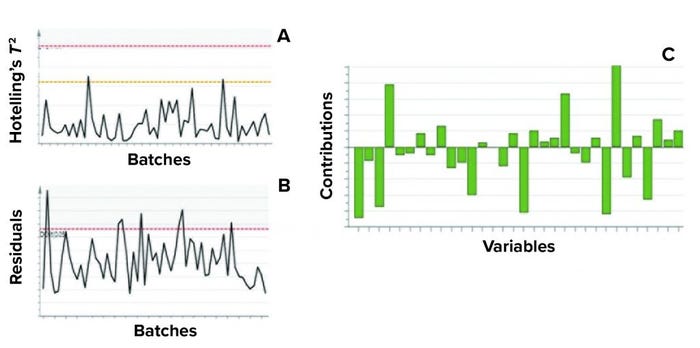
Figure 5: Example of model metrics used for excursion detection and diagnosis;
(a) Hotelling’s T² statistic and (b) model residuals are both used to identify excursions during process monitoring. (c) Contribution charts denote the contributions of variables toward an excursion for a batch, compared with the mean of all batches.

Model Training: After selecting the model structure with best performance — in this case, a PCA model considering all fill volumes together — the next step was to train the model. Model training here refers to the use of historical data to define control limits for multivariate metrics for process monitoring. Such multivariate control limits in turn would function as the “acceptable operating range” for future batches.

Process monitoring is facilitated using two multivariate metrics: Hotelling’s T² statistic and model residuals. Hotelling’s T² statistic represents the distance of an observation from the historical mean. Residuals refer to the part of a data set that cannot be explained by a model, usually noise in the data or an occurrence not seen by the model before. Acceptable ranges of Hotelling’s T² statistic and residuals for a batch is defined by the critical level of 95%. If a batch lies within the acceptable range for Hotelling’s T² statistic and/or residuals, then no action is taken. However, if a batch lies outside those acceptable ranges for either metric or both metrics, then further investigation of contributing factors is triggered.

Contribution plots provide a quantitative comparison of potential contributions for different process parameters toward a certain excursion. These plots show the difference of a selected batch (or group of batches) against the mean of all batches. Figure 5 shows an example of the two excursion-detection metrics (Hotelling’s T² statistic and model residual) and one diagnostic metric (variable contribution) for a model.

For model training, we used 45 batches in our analysis. All of those were considered for model training because they represent an acceptable operational range. That is because the quality of the DP was acceptable, so batches were not rejected. Batches used for model testing were excluded from the training data set.

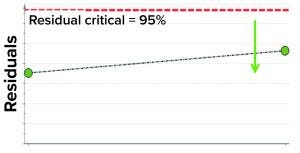
Figure 6: Model residual values for batches below (green arrow) the critical value of 95% (residual critical is shown in dashed red line) represent the batches that have similar correlation structure among the model parameters as the batches in the training data set.

Model Testing: MVDA models are tested to achieve two objectives. The first goal is to ensure that the models developed using a training data set are general enough to describe an independent data set. For that, we performed cross-validation to determine model complexity (number of principal components). The second goal is to demonstrate the model’s ability to capture correlations, detect excursions, and determine underlying contributing parameters.

For model benchmarking, we used two multivariate excursion-detection metrics: Hotelling T² range and residual. The objective of model benchmarking is twofold: to ascertain whether a model can capture correlations and to ensure that the model can detect excursions. To meet those two goals, we carried out model benchmarking in two steps.

In the first step, we removed two randomly selected “good” batches from the training data set and rebuilt the model. Both of those batches then were used as the test data set to assess whether the model could capture correlations. The model residual metric was used to test the model outcome. Model residual values for the two randomly selected “good” batches were below the multivariate critical limit for model residuals (red dashed line in Figure 6). Those results suggest that the two DP batches, which were tested against the model, have similar correlation structures among the model parameters as the batches in the training data set (Figure 6).

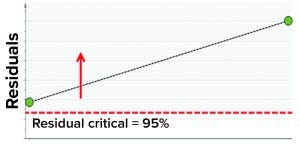
Figure 7: Model residual values for batches above (red arrow) the critical value of 95% (residual critical is the dashed red line) represent batches that have a correlation structure among the model parameters, which is different from the batches in the training data set.

In the second step, we used two batches known to have excursions as a test data set to ensure that the model could detect excursions. Residual values for both batches were beyond the critical limit, thus indicating that the batches had different correlation structures among the model parameters (because one or more had values different from the mean) from those in the training data set. Figure 7 shows that the “residual” multivariate diagnostic metric detected an excursion for a batch. Consequently, the contribution chart for the particular batch showed an abnormal value for fill-weight standard deviation. Examination of the univariate level showed the high values of fill weights caused by out-of-tolerance fill weight measurements (Figure 8). The corrective action for this excursion was recalibration of filling equipment. Such excursions (regardless of whether they influence a product) are worthwhile to detect and investigate as part of a holistic process-monitoring strategy.

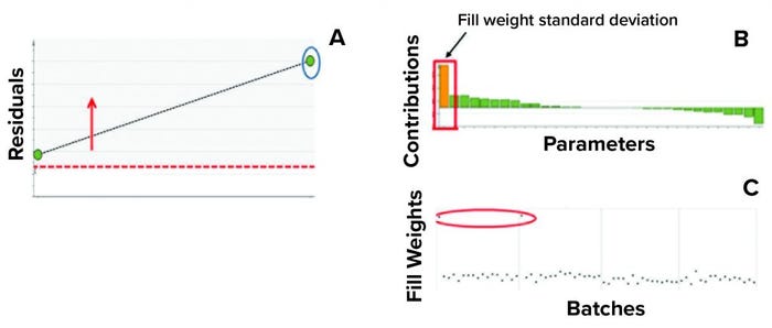
Figure 8: Using multivariate diagnostic metrics to find the root cause of an excursion requires multiple steps. (a) Diagnostic metric “residual” detects excursion for a batch (circled). (b) Contribution chart for the particular batch shows the abnormal value for fill- weight standard deviation. (c) Evaluations at the univariate level show the high values of fill weights. The process excursion detected here was caused by out-of-tolerance fill-weight measurement. The corrective action for this excursion was recalibration of the filling equipment.

Model Implementation: To enable use of such models for regular process monitoring, an appropriate information technology (IT) framework must be implemented. Such a framework needs to automate the following functionalities:

We developed and implemented such an environment based on the KNIME analytics platform (12). Two data analytics pipelines were implemented on the platform (Figure 9): one to automate model training and the other to evaluate new data against the trained model and generate an interactive report for end users. Our entire system was designed such that the complexity of data processing, model training, and execution is hidden from end users, and the results are easily accessible to them through interactive visualizations and reporting on a web browser.

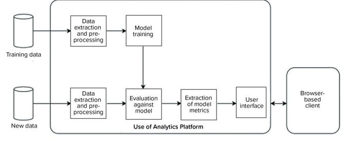
Figure 9: Overview of a data analytics platform for automated model training (top), evaluation of new data (bottom), and visualization

Benefits of Use
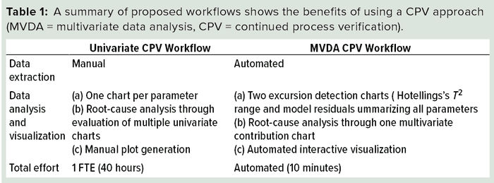
The proposed multivariate approach for CPV of FPM provides several benefits. Primarily, it helps in the identification of correlations among CQAs and CPPs for process monitoring. Implementation of the multivariate models on a web-based interactive platform increases its usability and the efficiency of data extraction and reporting analysis results. Root-cause analysis is an integral part of CPV that can be supported extensively by the multivariate platform. Table 1 lists an overview comparing traditional CPV and our proposed multivariate approach.

An Improved Strategy for CPV
CPV is an important requirement in biomanufacturing to ensure safe and efficacious therapeutic biologics. Implementation of a traditional CPV program that uses univariate analyses could consume excessive resources and time. That approach could be limited because CQAs and CPPs are assessed individually and not jointly, thus potentially excluding their interactions.

Effective MVDA methods monitor biomanufacturing processes and the corresponding product quality attributes. From a biomanufacturer’s standpoint, multivariate methods can streamline process monitoring operations while preserving the insights provided by using univariate analyses. Thus, implementation of MVDA in CPV programs offers an opportunity to improve their effectiveness and efficiency.

Our study focused on the development and implementation of MVDA for CPV in biomanufacturing. We developed MVDA models using historical data for CQAs and CPPs for a therapeutic protein. Those models were able to detect excursions. We also developed a pipeline for model implementation, increasing efficiency through automation and reducing the time required for report generation from ~40 hours to 10 minutes.

Although the utility of the MVDA CPV approach was demonstrated for an FPM process, the approach described herein can be extended to other process areas (e.g., upstream) and can be leveraged as a framework across multiple biologic therapeutics.

Acknowledgments
We thank colleagues from Manufacturing Sciences and Technology, who supported this effort.

References
1 Guidance for Industry: Process Validation — General Principles and Practices. US Food and Drug Administration: Silver Spring, MD, 2011; https://www.fda.gov/files/drugs/published/Process-Validation–General-Principles-and-Practices.pdf.

2 Rathore AS, Bhushan N, Sandip H. Chemometrics Applications in Biotech Processes: A Review. Biotechnol. Prog. 27(2) 2011: 307–315; https://doi.org/10.1002/btpr.561.

3 Kourti T. Multivariate Dynamic Data Modeling for Analysis and Statistical Process Control of Batch Processes. J. Chemomet. 17(1) 2003: 93–109; https://doi.org/10.1002/CEM.778.

4 Wold S, et al. The Chemometric Analysis of Point and Dynamic Data in Pharmaceutical and Biotech Production (PAT): Some Objectives and Approaches. Chemomet. Intell. Lab. Sys. 84(1–2) 2006: 159–163; https://doi.org/10.1016/j.chemolab.2006.04.024.

5 Kirdar AO, et al. Application of Multivariate Analysis Toward Biotech Processes: Case Study of a Cell-Culture Unit Operation. Biotechnol. Prog. 23(1) 2007: 61–67; https://doi.org/10.1021/bp060377u.

6 PAT: A Framework for Innovative Pharmaceutical Development, Manufacturing, and Quality Assurance — Guidance for Industry. US Food and Drug Administration: Silver Spring, MD, 2004; https://www.fda.gov/regulatory-information/search-fda-guidance-documents/pat-framework-innovative-pharmaceutical-development-manufacturing-and-quality-assurance.

7 Q8(R2). Guidance for Industry: Pharmaceutical Development. US Food and Drug Administration: Silver Spring, MD, 2009; https://www.fda.gov/regulatory-information/search-fda-guidance-documents/q8r2-pharmaceutical-development.

8 European Pharmacopoeia: Adoption of a New General Chapter on Multivariate Statistical Process Control. European Directorate for the Quality of Medicines and HealthCare, 11 May 2020; https://www.edqm.eu/en/news/european-pharmacopoeia-adoption-new-general-chapter-multivariate-statistical-process-control.

9 Discoverant User’s Guide. Aegis Analytical Corporation, 2001; http://pearsontechcomm.com/samples/Discoverant_Users_Guide.pdf.

10 Basilevsky A. Statistical Factor Analysis and Related Methods: Theory and Applications. John Wiley & Sons: Hoboken, NJ, 2009.

11 Eriksson L, et al. Multi- and Megavariate Data Analysis: Basic Principles and Applications. Umetrics Academy: Umeå, Sweden, 2013: 425.

12 Fillbrunn A, et al. KNIME for Reproducible Cross-Domain Analysis of Life Science Data. J. Biotechnol. 261, 2017: 149–156; http://doi.org/10.1016/j.jbiotec.2017.07.028.

Shreya Maiti is a senior scientist, Michal Mleczko is biotech digitalization lead, and corresponding author Konstantinos Spetsieris is head of data science and statistics, all at Bayer US LLC, 800 Dwight Way, Berkeley, CA 94710; 1-510-705-4783; [email protected]; http://www.bayer.com.