Biopharmaceutical Product Specification Limits and Autocorrelated Data

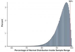
Figure 1: Percentage of normal distribution covered by the sample range, n = 30 with ACF(1) = 0

Calculations, including statistical tolerance intervals, can assist in the development and revision of specification acceptance criteria. Manufacturing results for attributes of a biopharmaceutical product can be positively autocorrelated. The sample standard deviation — calculated from limited, positively autocorrelated data — tends to underestimate the long-term process standard deviation (1). In this article, simulated data are used to assess the relative performance of statistical tolerance intervals, intervals calculated using the minimum process performance index P_pk approach, and the sample range.

Prevalence of Positively Autocorrelated Data
The estimate of process standard deviation (σ) calculated from a limited number of batches (n) can be markedly underestimated when data are positively autocorrelated. The presence of positive autocorrelation (values that are closely related to each other in sequential order) for a biopharmaceutical manufacturing process can be caused by a number of factors, including lack of sensitivity of an analytical method and homogeneity of input factors (e.g., multiple drug product batches sourced from a common drug substance lot). In a recent assessment, over 75% of quality attributes in continued process verification (CPV) activities for one biopharmaceutical product had lag-one sample autocorrelation function estimates between 0.0 and 0.5 (1). Therefore, analysts recommended using the sample standard deviation as the estimate of σ when at least n = 30 results are available for biopharmaceutical CPV activities (e.g., control charting).

Statistical Tolerance Intervals and Acceptance Criteria Determination
A statistical calculation such as a tolerance interval (2) can assist in the decision-making exercise for developing specification acceptance criteria (SAC). One aim is to find reasonable limits to represent expected results from a current manufacturing process. That information is used with nonstatistical considerations, including clinical experience, to determine SAC. Before a drug product is commercialized, SAC-related calculations may involve fewer than 30 batches.

Consider a situation in which n = 10 drug product lots have been manufactured. To obtain an interval in which a large proportion of individual values would fall, a two-sided 95% confidence/99% coverage tolerance interval (95/99 TI) is calculated as the sample mean ± 4.44 sample standard deviation when assuming a normal distribution (3). That interval covers at least 99% of individual values with 95% confidence (95% of the time).

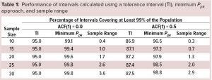Monte Carlo simulations as described in a previous study (1) were performed using 108 samples for each value of n to assess the long-run relative frequency (confidence level) for which at least 99% of individual results were contained inside the interval. For example, generating independent data (autocorrelation function, ACF(1) = 0) and calculating two-sided 95/99 TIs using the TI multipliers for 95% confidence as described by Hahn and Meeker (3), the confidence level for 99% coverage is, as expected, 95.0% for each sample size (Table 1). However, if data are positively autocorrelated with ACF(1) = 0.5, then the achieved confidence level with n = 10 is not 95.0% but about 86.9%. Therefore, TIs have lower confidence levels than expected when limited data are positively autocorrelated, and this includes the situation in which n = 30.

Minimum P_pk and Sample Range Intervals
Another calculation strategy to assist in determining specification acceptance criteria  the minimum P_pk approach (4). This approach uses the sample size, sample mean, and sample standard deviation to generate an interval such that the lower bound of an approximate two-sided 95% confidence interval for P_pk is ≥1. This approach tends to generate intervals closer to a 95/99 TI when encountering positively autocorrelated data (Table 1). For example, with n = 10, when results are positively autocorrelated with ACF(1) = 0.5, this interval would correspond to a 96.5/99 TI.

Simulations also were performed to assess sample range, namely the difference between the largest and smallest results of a sample of size n. The conclusion from that analysis is that practitioners would be ill-advised to use sample range to assist in setting SAC because of the low confidence levels for capturing a high percentage of the distribution. For example, when n = 10, the achieved confidence level is only 0.4% with independent results and 0.3% when results are positively autocorrelated with ACF(1) = 0.5 for 99% coverage. That should not be surprising, because it can be shown that the expected percentage of the distribution to be covered by the sample range using independent results equals (n – 1)/(n + 1) (5). Thus, with n = 30 independent results, the average percentage covered by the sample range is 100 (29/31)% ≈ 93.5%. The sample range calculated using n = 30 is equivalent to only a 3.6/99 TI (Table 1) and illustrated using simulated results in Figure 1.

Practical Implications for Specification Acceptance Criteria Determination
Positively autocorrelated data are likely to be used in calculations to assist in developing SAC for a biopharmaceutical manufacturing system. A TI calculated using limited amounts of such data provides intervals with a lower confidence level than expected. The minimum P_pk approach guarantees that the calculated interval is such that the lower two-sided 95% confidence bound of P_pk is at least one, and it has further been illustrated to provide intervals closer to the expected performance of 95/99 TIs with positively autocorrelated data. Use of a sample range to assist in SAC calculations has been shown to lack adequate confidence for high coverage levels and thus is not recommended.

References
1 Bower KM. Determining Control Chart Limits for Continued Process Verification with Autocorrelated Data. BioProcess Int. 17(4) 2019: 14–16.

2 Dong X, Tsong Y, Shen M. Statistical Considerations in Setting Product Specifications. J. Biopharm. Statistics 25, 2015: 280–294.

3 Hahn GJ, Meeker WQ. Statistical Intervals: A Guide for Practitioners. John Wiley & Sons: Hoboken, NJ, 1991; 291.

4 Coffey T, Bower KM. A Statistical Approach to Assess and Justify Potential Product Specifications. BioProcess Int. 15(2) 2017: 38–39.

5 Mood AF. Introduction to the Theory of Statistics. McGraw-Hill: New York, NY, 1950; 387.

Keith M. Bower, MS, is senior principal CMC statistician at Seattle Genetics, Inc. and an affiliate assistant professor in the Department of Pharmacy at the University of Washington; [email protected]; www.seattlegenetics.com.

SAS Enterprise Guide 7.15 was used to calculate the results for Table 1 and to generate Figure 1.