The Relationship Between R2 and Precision in Bioassay Validation

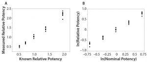
Figure 1: Simple linear regression analyses using original data and logarithm base e transformed data; (LEFT) bivariate fit of measured relative potency by nominal potency; (RIGHT) bivariate fit of ln(relative potency) by ln(nominal potency)

Analytical linearity along with assessments of precision and accuracy determine the range for bioassays (1). Practitioners can include coefficient of determination (R²) criteria from a linearity study in the bioassay validation protocol. Herein I illustrate the relationship of R² to study design and analytical method variation.

Overview of the Simple Linear Regression Model
Dilutional linearity assesses the “ability (within a given range) of a bioassay to obtain measured relative potencies that are directly proportional to the true relative potency of the samples” (1). With bioassay data, a logarithm base e data transformation provides the appropriate use of a simple linear regression model by reducing the impact of variance heterogeneity with increasing potency (2). The assumed linear relationship between ln(relative potency) and ln(nominal potency) can be assessed using Equation 1.

Equations:

The method of ordinary least squares can be used to estimate unknown coefficients (intercept and slope). R² compares the total variation (SS_total) with the variation not explained by the model (SS_error), as shown in Equation 2 (3). With a simple linear regression model, if the value of R² is one, the results lie on a perfectly straight line. But an R2 value of zero does not necessarily imply no relationship (4).

Illustration of Linearity and Precision Calculations
Here I use data from USP <1033> to calculate assessment of linearity (5). As described in USP <1033>, results from a linearity study also can be used to estimate bioassay precision and accuracy. Eight assays (two analysts, four runs per analyst) are performed at five nominal potency levels (0.50, 0.71, 1.00, 1.41, and 2.00). Use of a logarithm base e transformation on all data is justified to provide similar variation across an assessed range (Figure 1).

After fitting the regression line using Equation 1, R² is calculated as 1 – (0.15213/10.57003) = 0.986. So the regression model using transformed data explains about 98.6% of total variation. Intermediate precision can be assessed using percentage of coefficient of variation (%CV). With logarithm base e transformed data, CV% can be calculated using Equation 3 (5).

From the linearity study, the mean square error (MSE) is calculated as SS_error/(n – 2) and represents “average” variation across the range. This result can be substituted for SD_Ln² in Equation 3. For example, the “average” %CV from this linearity study is 100 × √(exp(0.15213/38) – 1)) ≈ 6.3%.

Relationship Between R² and CV%
The relationship between R² and %CV in a linearity study can be expressed using simulated data. For this study, a programmer executes the following steps:

Step 1: Generate eight values for each nominal potency level (0.50, 0.71, 1.00, 1.41, 2.00).

Step 2: Transform each value in step 1 using logarithm base e. These will be the ln(nominal potency) values.

Step 3: Calculate 40 random values from a normal distribution with zero mean and standard deviation value between 0.05 and 0.15. These values represent various levels of assay intermediate precision.

Step 4: Sum the values from steps 2 and 3. These will be the ln(relative potency) values.

Step 5: Using the method of ordinary least squares, calculate the MSE and R² results using the values in steps 2 and 4 with Equation 1.

Step 6: Using the MSE from step 5, calculate the “average” %CV using Equation 3.

Step 7: Repeat steps 1–6 to build a library of simulated results.

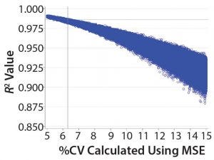
Figure 2: Values of R² calculated from simulated data with different levels of precision

Figure 2 shows the relationship between the “average” %CV and R² results for the USP <1033> linearity study. The values of %CV = 6.3% and R² = 0.986 are superimposed on the graph as a reference. Note that for this linearity study design, a validation criterion of R² ≥0.95 always would be met if the “average” method intermediate precision has %CV <9%.

This type of statistical risk assessment is recommended for practitioners seeking to use predefined R² criteria in a validation protocol. A follow-up article next month will address implementing multiple acceptance criteria (including R²) in a validation exercise and understanding the effect of the experimental design on expected outcomes.

References
1 USP <1030> Biological Assays Chapters — Overview and Glossary: IV Terms Related to Validation. USP 40–NF 35. United States Pharmacopeial Convention: Rockville, MD, 2017.

2 USP <1032> Design and Development of Biological Assays, Section 4.3. USP 40–NF 35. United States Pharmacopeial Convention: Rockville, MD, 2017.

3 Hogg RV, Ledolter J. Applied Statistics for Engineers and Physical Scientists. 2nd ed. Jonh Wiley and Sons, Inc.: New York, NY, 1992.

4 Colton JA, Bower KM. Some Misconceptions About R². International Society of Six Sigma Professionals, EXTRAOrdinary Sense 3(2) 2002: 20–22.

5 USP <1033> Biological Assay Validation. USP 40–NF 35. The United States Pharmacopeial Convention: Rockville, MD, 2017.

Keith M. Bower, MS, is principal CMC statistician at Seattle Genetics, Inc. SAS Enterprise Guide 7.12 software was used to simulated bioassay results and generate Figure 2. JMP v13 software was used to generate Figure 1.