Run Rules with Autocorrelated Data for Continued Process Verification

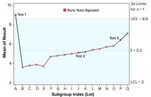
Figure 1: Individuals (X) chart of results; subgroup sizes n = 1; UCL = upper control limit, LCL = lower control limit

Control charts can be used to assist in monitoring of biopharmaceutical product quality attributes as part of continued process verification activities. A number of tests known as run rules have been developed to assess whether biomanufacturing processes remain in statistical control. In practice, results for such attributes can be positively autocorrelated. Simulated data are used to assess the performance of run rules with autocorrelated data to assist in determining risk–reward profiles for process monitoring.

Autocorrelated Data
The tendency for data to be positively autocorrelated (values are closely related to each other in sequential order) in biopharmaceutical manufacturing processes and the effect of such data on the performance of run rules have been highlighted in two 2019 studies (1, 2). The simulation strategy used herein is based on a Monte Carlo approach to represent how autocorrelated data affect the usefulness of combinations of run rules with Shewhart individuals control charts (X charts) as part of an overall control strategy.

Run Rules and Recommendations for Their Use
Using tests to assess the behavior of results in a control chart was addressed in Western Electric’s Statistical Quality Control Handbook (3). Lloyd Nelson’s technical note added tests, along with suggesting minor alterations to earlier tests (4). The ICH Q9 guideline recommends that the “level of effort, formality, and documentation of the quality risk management process should be commensurate with the level of risk” (5).

However, it does not include recommendations on which run rules should be used. With the availability of statistical software for control charting, practitioners might be tempted to apply all eight of Nelson’s tests without considering the practical consequences (6). Nelson suggested that “tests 1, 2, 3, and 4 be applied by the person plotting the chart.”

Those four tests are known as Nel 1 to Nel 4 and described below.

Nel 1: One point is above or below the three-sigma control-chart limits (to detect a large shift in process mean or a one-off “error” such as an incorrect data entry).

Nel 2: Nine points in a row are on the same side of the centerline (to detect a sustained shift in the process mean such as switching to a different raw material source).

Nel 3: Six points in a row are increasing or decreasing steadily (to detect an increasing or decreasing trend/drift such as those caused by decreasing analytical method variation with increasing experience running the assay).

Nel 4: Fourteen points in a row are alternating up and down (to detect nonrandom systematic variation; for example, two operators used alternately).

To illustrate run tests using SAS software, Nel 1–4 were selected to assess data provided in Table 1 and Figure 1. Assume that prior knowledge recommends use of 5.3 as the centerline to represent the process mean, and the process standard deviation is assumed to be 1.1. Thus, limits in the X chart are 5.3 – 3(1.1) = 2.0 for the lower control limit (LCL), and 5.3 + 3(1.1) = 8.6 for the upper control limit (UCL).

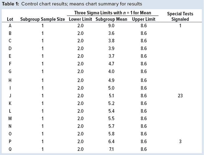
Note that Nel 1 is flagged for lot A. Both Nel 2 and Nel 3 signal for lot J, but only one test (Nel 2) is indicated in the X chart. Although the data continue to increase, unbroken data trend from lots K and onward, and Nel 3 does not signal again until lot P. That follows Nelson’s recommendation to flag at “the last [point] of a sequence of points (a single point in Test 1) that is very unlikely to occur if the process is in statistical control.”

This aspect of signaling leads to slight differences between results in this article and other publications. However, it more closely reflects run-rule use in the biopharmaceutical industry; namely, to address a potential special cause when it first appears.

Probability of False Alarms
The Monte Carlo approach as described in a previous study (1) used one billion data values for each simulation, generating data with lag 1 autocorrelation function (ACF(1)) values from 0 (no autocorrelation, hence independent results) to 0.5, in increments of 0.1. The probability of exceeding one test (or more) for a given lot can be calculated by summing the total number of lots associated with one or more signals and dividing that value by one billion. Note that the interest is only in whether a signal exists for a given lot rather than how many tests are signaling. For example, assuming independent normally distributed results (ACF(1) = 0), the probability of a Nel 1 signal by chance alone (a false alarm) is 1 – 0.9973, or 0.27% of the time. Practically, a lot with one or more signals is assessed by quality control to determine whether a process remains in a state of control. Such conclusions typically are summarized in an annual product review, which must be conducted at least annually per the Code of Federal Regulations for commercial products (7).

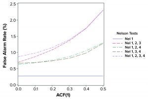
Figure 2: False alarm rates in relation to Nelson tests and autocorrelation (ACF = autocorrection function)

Relative Performance in Relation to the Level of Autocorrelation
The population mean and standard deviation were used to calculate the control chart limits for each simulation, following the approach in a previous study (1). Simulated data are assumed to represent an in-control process. Table 2 and Figure 2 show how false-alarm rates change with increasing serial dependence and an increasing number of tests. For independent results, when including either Nel 2, 3, or 4 to Nel 1 in the family of tests, the false-alarm rate roughly doubles. As expected, Nel 4 is less likely to signal when values are more closely related (with increasing positive autocorrelation). Thus, a false-alarm rate will be influenced more by the other tests being used in the combination of run rules.

Practical Implications for Run Rule Usage
Positively autocorrelated data can be analyzed as part of continued process verification activities for a biomanufacturing system. As more tests are used, the probability of a false-alarm increases. The likelihood of a false-alarm also increases with increasing positive correlation in data when incorporating more tests (other than Nel 4). If a company’s control-charting strategy for continued process verification uses Nel 1–4, a false alarm can be expected roughly 0.87% of the time when data are independent. However, when data are positively autocorrelated with ACF(1) = 0.5, a false signal can be expected 2.30% of the time. Practitioners are advised to consider the implications of false-alarm rates for control charts when developing their continued process verification strategy.

References
1 Bower KM. Determining Control Chart Limits for Continued Process Verification with Autocorrelated Data. BioProcess Int. 17(4) 2019: 14–16.

2 Oh J, Weiß CH. On the Individuals Chart with Supplementary Runs Rules under Serial Dependence. Methodol. Comput. Appl. Probab. 22, 2019: 1257–1273; https://doi.org/10.1007/s11009-019-09760-2.

3 Statistical Quality Control Handbook. Western Electric, American Telephone and Telegraph Company: Chicago, IL, 1956.

4 Nelson LS. The Shewhart Control Chart: Tests for Special Causes. J. Qual. Technol. 16(4) 1984: 237–239; https://doi.org/10.1080/00224065.1984.11978921.

5 ICH Q9: Quality Risk Management. Fed. Register 71, 2005: 32105–32106.

6 Hare LB. Follow the Rules: Don’t Dismiss the Nelson Rules When Looking for Causes of Variation. Quality Progress. American Society for Quality: Milwaukee, WI, 2013.

7 Code of Federal Regulations, Title 21, Vol. 4, Sec. 211.180. 2020.

Keith M. Bower, MS, is a senior principal scientist in CMC statistics at Seagen, Inc. (formerly Seattle Genetics), and an affiliate assistant professor in the Department of Pharmacy at the University of Washington; [email protected]; www.seagen.com.

SAS v9.4 was used to calculate results for Tables 1 and 2 and to generate Figures 1 and 2.