Model Predictive Control for Bioprocess Forecasting and Optimization

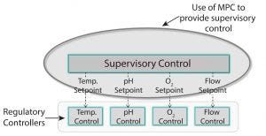
Figure 1: In the automation hierarchy, base level of regulatory control maintains process variables at setpoints (single-input-single-output, SISO) and PID or programmable logic control (PLC) methods. Model predictive control (MPC) provides supervisory control of future variable trajectories and final batch conditions. Advanced supervisory control allows base-level control setpoints to achieve quality or economic objectives (multiple-input-multiple-output, MIMO).

Automation hierarchy in bioprocess manufacturing consists of a regulatory layer, process analytics technology (PAT), and (potentially) a top-level model-predictive or supervisory layer. The regulatory layer is responsible for keeping typical process measurements such as temperature, pressure, flows, and pH on target. In some cases, spectral instrumentation in combination with multivariate analysis (MVA) can be configured to measure parameters such as glucose concentration. A cascade control structure can be set up when the nutrient flow setpoint is adjusted to maintain the reactor glucose concentration at a specified target value. On top of the regulatory and supervisory layers, a supervisory control layer can be used to determine optimal trajectories for glucose, temperatures, pH, and so on to optimize cell growth or productivity kinetics and final batch conditions.

Toward Supervisory Control
PAT, soft sensors, and inferential controls are enabling technologies to observe and maintain a process at a consistent state. They are strong foundations to enable process capability — which allow us to make processes do what we want them to do. We can control parameters such as glucose, temperature, pH, and other factors. Basically, if we can measure it, we can control it. For example, if we can control glucose, then we can consider what that glucose profile should be to maximize titer and other conditions at batch completion. Moving from PAT to supervisory control with model predictive control (MPC) goes beyond process capability and into product quality and process optimization (Figure 1).

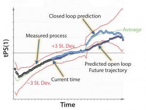
Figure 2: Example of model predictive control (MPC); predictive modeling is used to detect and mitigate process deviations before they happen.

To optimize bioprocesses, manufacturers are moving from descriptive and diagnostic analytics (determining what and why an action happened) to predictive analytics (determining what will happen) and, ultimately, prescriptive analytics (making something happen or not happen). Progressing higher in that “analytics food chain” requires automation, making smart decisions, and building processes that optimize themselves (Figure 2).

One approach that has become common in biologics manufacturing is the use of multivariate modeling and calibrate models to determine how a process should run. We turn such models into control charts and track a process as it is running. But a better approach (related to MPC) is to ask, “Based on how cells are responding and the process is running, can we predict where the process is going? If we can forecast and we have good models, can we then optimize? Is there an adjustment that we can make so that the process follows the path that we want it to run? How do we then predict the future?” Right now, the turnkey strategy is to use imputation methods. In the future, biomanufacturing industry would benefit from using a “hybrid” approach — using both data-driven aspects and mechanistic understanding.

Imputation Methods
Imputation has been around for 20 years and is still a good tool because it works very well. Figure 3 shows a simple example. If we measure two parameters that are correlated, what happens if we only measure one so that some data are missing? We want to understand, where the process “lives” in a scatter of data. If we think of the data as a calibration curve, we can see that there is correlation, and can fit a line to it, project to this line, and then estimate where the missing data are likely to be.

Consider what happens in a process: Let’s say that you have a 14-day cycle, and you have collected data from the first day or two. The cells reveal themselves very quickly, so you can see how they are growing right away. You don’t need to measure the entire batch to understand what type of growth is happening for this particular batch. This means that at the beginning of the run, you can look at the signature of how the cells are growing and how they are responding to media and other factors. With the right approach, you then can project what the rest of the growth profile will look like. Once the beginning of the run has been measured, you can look at your calibration curve for the process and evaluate where you expect the end to be. That is imputation.

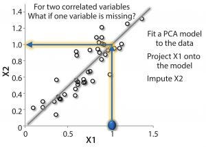
Figure 3: Simple example of imputation; for two correlated variables (X1 and X2), use PCA/PLS model as a calibration curve of the system. If one component is missing, the other can be projected onto the model, and the missing component can be imputed (e.g., X2 = 1).

By using partial least squares (PLS), process controls and automation, and multivariate-type models, we can do exactly that. The details of doing so using many different methods are beyond the scope of this article but some have been described in the literature (1). In general, the steps are quite simple. First, build a model and use a software system such as SIMCA (Umetrics, now Sartorus Stedim Data Analytics AB; Control Advisor in SIMCA-online uses a patented imputation method that uses PLS regression — imputation by regression, IBR — which is a comparable or even better method than iterative methods and computationally efficient for optimization) (2, 3). With those measurements, you can estimate “scores” in the model. Based on those estimations, you can fill in the missing data (imputation). Ideally, you want to invert the model. The mathematical analogy is that you read the measurements you have, correlate them with existing data, and then read off that missing data (Figure 3).

What do we do with that method? In Figure 2, the red lines are control limits, and the green line is what is commonly referred to as a golden batch. We measure up to the current time point, then use imputation to project where the process is expected to go based on the current time point and where it will go in the future.

If we can predict, and we have the right type of models, then we can optimize. Optimization of our model allows us to change our setpoints (e.g., for glucose). With that change in the glucose setpoint, we can observe the response we get from the cells. Then we can put that type of modeling structure inside of an optimization loop or optimizer — basically, model predictive control. MPC uses a model of a process inside an optimization routine to decide how a process should run.

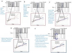
Figure 4: Optimization with model predictive control (MPC)

Figure 4 shows how optimization with MPC works. First, we calibrate a multivariate model based on historical data. Data are collected for a batch that is currently running (X_K) (Figure 4A), and future trajectories of the dependent variables (X_D) are estimated using imputation (Figure 4B). Some of future settings are known; they are assignable (Figure 4C). Such parameters are the manipulated variables (X_MV) such as glucose setpoint. An optimization routine is used to iterate through various combinations of future X_MV values to converge on the optimal set (this is MPC).

Figure 4E summarizes this process: We hypothesize a set of future setpoints (X_MV), which could be our recipe as a starting point. We use imputation to fill in where we expect the process to go with that recipe. “Evaluate process” basically means to calculate final conditions such as peak titer, final viable cell density, or whatever other criteria to evaluate how well or poorly the process ran (final qualities and so on). Then we try a new set of manipulative variables and keep iterating until we find the set that optimizes the process.

The purpose of the regulatory layer of process automation (which includes PAT and inferential control) is to establish process consistency and capability as well as to provide a foundation for advanced control. We want the process to follow a certain trajectory, and we want to know that it will follow that trajectory. With tools such as MPC, we can now determine the economic optimization and quality performance. It is the top level on the hierarchy that we are trying to achieve. You can’t conduct supervisory control and thus optimization without having a well-performing regulatory foundation layer first. Those systems (regulatory and supervisory) do not fight or compete with each other; they are complementary. The regulatory layer focuses on the process, and supervisory control focuses on quality and performance. You can’t do one without the other.

Disruptive Technologies
Data-driven approaches are useful, they have their roles — but they are not everything. We need also to leverage our mechanistic understandings. Both modeling approaches complement each other. My idea is to put together an advanced monitoring toolkit. With the ability to select instrumentation in a process (determining the different pieces), biomanufacturers can come up with the set of measurements needed to provide observability to support modeling efforts. By doing so, not only can they monitor what they are measuring, but also translate that information into what they are interested in. They also can build “state observers” that get them a little closer to quality. Basically, they can translate the parameters that they measure into those that they are interested in by using the mechanistic modeling forms that track mass, energy balance, and kinetic information.

Researchers are working on scale-independent modeling (e.g., taking in more mixing characteristics) so that we can take a model built on a small scale and then use it in at larger scales. Ultimately, the goal is to have a system that monitors how cells are performing and what is going on inside the cells. The idea is to have more intelligent monitoring. If we want to control and have better types of automation and control, we need “observability.”

That is where we are moving now in bioprocessing. We need to be able to see what is going on at an in-depth level. We need to see what is going on inside of cells and not know simple parameters such as pH and so on, but rather see at much higher levels. At Sartorius-Stedim Data Analytics, we have skill sets in many different areas. We are at a turning point where these are not just ideas about what we could do, but there is also a pull from industry. We are moving much more toward machine learning, deep learning, artificial intelligence, and so on, for example.

In terms of our development roadmap, the products we sell are Windows-based products, but we recognize that this way of delivering products will not going be the way that people want or need to have their tools delivered in the future. So our analytics core runs in other types of environments. There is a consensus, in how that needs to happen. And we are thinking of data in different ways — not just as numbers, but also text, images, and information that can be found in many different places. You can take information and apply machine learning and deep-learning applications to get nontraditional types of information, summarized in nice ways. Taking these ideas and bringing them into manufacturing is an area of keen interest for us.

References
1 Arteaga F, Ferrer A. Dealing with Missing Data in MSPC: Several Methods, Different Interpretations, Some Examples. J. Chemometrics 16(8–10) 2002: 408–418; doi:10.1002/cem.750.

2 Garcia-Munoz S, Kourti T, MacGregor J. Model Predictive Monitoring for Batch Processes. Ind. Eng. Chem. Res. 43(18) 2004: 5929–5941; doi:10.1021/ie034020w.

3 Nomikos P, MacGregor J. Multivariate SPC Charts for Monitoring Batch Processes. Technometrics 37, 1995: 41–59; doi:10.1080/00401706.1995.10485888.

Chris McCready is a lead data scientist at Sartorius Stedim Data Analytics, participating in R&D and development and deployment of data analytical solutions in the biopharmaceutical and other industries; [email protected].

This article is based on a presentation at Biotech Week Boston, 24–27 September 2017.