Using Prior Knowledge to Estimate Long-Term Variation

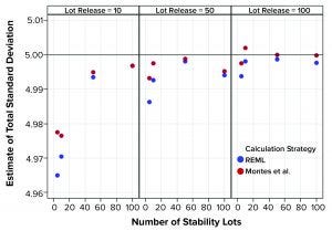
Figure 1: Estimates of total standard deviation from simulated results; REML is restricted maximum likelihood, and Montes et al. is in Reference 1.

A reasonable estimate of long-term variation for a biopharmaceutical product critical quality attribute (CQA) can be challenging to justify, especially in the early stages of a product’s lifecycle when only limited data are available. However, if the combination of product and analytical method reasonably can be matched with historical data, prior knowledge can provide an estimate of a value. This variation estimate could be used to assist in risk assessments related to continued process verification (CPV) activities, including control charting and estimating manufacturing capability. The study below uses simulated data to suggest a calculation strategy for analyzing prior-knowledge data, with estimates of variance components.

Sources of Variation
When estimating the total variance for a CQA, analysts should include stability data (at the recommended storage condition) with lot-release data to model appropriately the expected behavior of an attribute over a product’s shelf life. The positive square root of the total variance is the total standard deviation, which expresses variation in the original units of the metric. As the amount of data increases, analysts can obtain a more appropriate representation of long-term variation and make estimates of individual sources of variation that comprise total variance. The strategy described in Montes et al. (1) combines two datasets: lot-release data, which are values solely at t = 0 months, and stability data. Stability data are test results taken at predetermined time points for a manufactured lot in a stability study.

The mixed-effects model used by Montes et al. for an attribute that changes with time assumes a common fixed rate of change over time across lots, where Lot is a random effect and takes the form of

Y_ij = µ + Lot_i + β × Time_ij + E_ij

In that equation, i = 1, . . . I lots; j = 1, . . . J_i time points for lot i; Lot_i is normally distributed with a mean of zero and standard deviation σ_L. E_ij is normally distributed with mean of zero and standard deviation σ_E.

Lot_i and E_ij are independent. So, the response variable Y_ij has standard deviation σ_Total = (σ²_L + σ²_E)^1/2. Note that σ²_E represents analytical method variance. Seagen analysts assessed the applicability of this model using commercial and late-stage products manufactured by Seagen and its partners. The mixed-effects model was useful, with the residuals tending to be well behaved for many of the CQAs assessed. Where the model did not fit adequately, that was caused primarily by the lack of the number of distinct results available in the dataset (e.g., fewer than five distinct results for an attribute).
When following the calculation strategy of Montes et al. and comparing the relative importance of the estimates of the variance components σ²_L and σ²_E to σ²_Total, the findings frequently disagreed with the expected outcome based on considering prior knowledge.

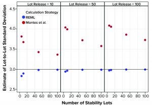
Figure 2: Estimates of lot-to-lot variation from simulated results; REML is restricted maximum likelihood, and Montes et al. is in Reference 1.

Comparison Study
Analysts compared the calculation strategy described by Montes et al. and results using the method of restricted maximum likelihood (REML) available in SAS software (2). Ten thousand simulations were used for different combinations of lot-release values and stability lots (with six time points per stability lot). Data were simulated such that the standard deviation for the analytical method (σ_E) was 4, and σ_L = 3. So, σ_Total = (4² + 3²)^1/2 = 5. The number of lot-release tests assessed were 10, 50, and 100, which was in conjunction with 5, 10, 50, and 100 stability lots. The simulations provided an opportunity to assess the statistical performance early through mature stages of manufacturing.

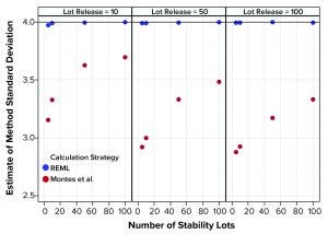
Figure 3: Estimates of method variation from simulated results (REML = restricted maximum likelihood, Montes et al. is Reference 1)

Figure 1 shows that the calculation approach used by Montes et al. (1) provided an estimate of σ_Total, which was at least as good as the REML result. The estimates were very close to the actual value σ_Total = 5. However, the estimates of σ_L and σ_E in Figures 2 and 3, respectively, using the approach from Montes et al. can differ markedly from the correct values. By contrast, the REML calculation generated estimates of σ_L and σ_E that were very close to the correct values. Notably, the aim of the calculation strategy in Montes et al. was to provide a useful, easy-to-calculate estimate of σ²_Total to be used in the calculation of statistical tolerance intervals. The goal was not to provide appropriate estimates of the constituent sources of variation.

Based on those findings, the calculation strategy used by Montes et al. is recommended to obtain estimates of σ²_Total (hence σ_Total). That strategy is useful especially when encountering unbalanced designs, including situations in which stability and lot-release data are combined. However, if the goal is to calculate estimates of σ_L or σ_E to understand the percentage of variation attributable to each source of variation, then the REML approach is recommended.

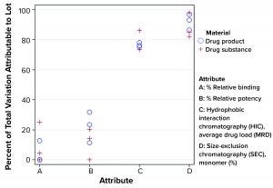
Figure 4: Percentage of total variation attributable to lot-to-lot variation

Practical Use of Variance Component Estimates
Using the model from Montes et al., σ_2Total can be estimated using the variance component estimates from REML, in which σ_2Total = σ_2L + σ²_E. Using prior knowledge, namely the combination of lot release and stability data, the percentage of the estimate of σ_2Total attributed to σ_2L tended to be relatively consistent within each attribute. That was regardless of the number of manufactured lots using the Seagen data. Figure 4 shows that from a subset of all CQAs assessed, that percentage can differ markedly across attributes. By identifying such behavior, analysts can be aware of an “expected” long-term variation as it relates to the relative importance of lot-to-lot and analytical method variation. That strategy should lead to more appropriate estimates of long-term variation than those obtained by using a somewhat arbitrary multiple of analytical method variation from a method-qualification exercise.

References
1 Montes RO, Burdick RK, Leblond DJ. Simple Approach to Calculate Random Effects Model Tolerance Intervals to Set Release and Shelf-Life Specification Limits of Pharmaceutical Products. PDA J. Pharm. Sci. Technol. 73(1) 2019: 39–59; https://doi.org/10.5731/pdajpst.2018.008839.

2 Dickey DA. PROC MIXED: Underlying Ideas with Examples. SAS Global Forum 2008, paper 374-2008; https://support.sas.com/resources/papers/proceedings/pdfs/sgf2008/374-2008.pdf.

Keith M. Bower, MS, is a senior principal scientist in CMC statistics at Seagen Inc.; [email protected]; www.seagen.com.