Choosing Tolerance Intervals: A Framework To Use in Setting Specification Limits Based on Manufactured Drug Lot Data

HTTPS://WWW.ISTOCKPHOTO.COM

As defined in ICH Q6A, a specification is a list of tests, references to analytical procedures, and appropriate acceptance criteria that take the form of numerical limits, ranges, or other criteria for the tests described (1). They establish the set of criteria to which a new drug substance or product should conform to be considered acceptable for its intended use.

Ideally, specifications are established based on demonstration of quality attribute levels that make drugs safe and efficacious during toxicology and clinical studies. At that point in development, however, analytical and process variability may not be reflected fully by the few drug lots used for such studies. Along with test data from toxicology and clinical studies, ICH Q6A cites relevant development data, pharmacopeial standards, and results from accelerated and long-term stability studies, as justification of specifications. Additionally, the guideline states that companies should take a reasonable range of expected analytical and process variability into consideration.

Tolerance Interval Overview
A tolerance interval (TI) is defined as an interval that can be claimed to contain at least a proportion (P) of the population with a specified degree of confidence (γ). Because a TI is an inference of the distribution, it can be used as a statistical tool to set pharmaceutical drug-product specifications (2, 3). When a TI is calculated from drug-lot data, it incorporates estimates of analytical and process variability as ICH Q6A recommends.

A calculated TI can provide a starting point for stakeholders who are tasked with establishing specification limits. To bracket practically an entire population, P = 0.9973 is used for the normal distribution. A confidence level of γ = 0.95 is used traditionally to control type I (false positive) errors at α = 0.05. The TI method is calibrated to maintain γ for a targeted P and sample size (n). When n is small, the TI will be commensurately wide to compensate for the large sampling uncertainty and maintain γ = 0.95 while bracketing
P = 0.9973. Some practitioners choose to operationalize that n, γ, and P relationship by arbitrarily choosing

• P = 0.9973 for n ≥ 30
• P = 0.99 for 15 < n < 30
• P = 0.95 for n ≤ 15.

The mathematical formula for a TI depends on a number of factors:

• assumed distribution of the population from which sampled lots are drawn (e.g., normal, lognormal, and gamma)
• structure of sampled data — univariate (a single measurement per lot from release-only data) or hierarchical (multiple measurements over time per lot from stability data)
• nature of the quality attribute (stability-indicating or not, and changing linearly or nonlinearly over time)
• reporting of measurements relative to the limit of quantitation (LoQ), whether fully observed (above LoQ) or left-censored (below LoQ).

So even though TI is a straightforward concept by definition, quality analysts have to work through a number of decision forks to identify which formula to choose and then look for available computing tools to apply for the chosen TI type. This article can help practitioners do so by providing decision-tree diagrams and quick-guide computing resources. This is a high-level framework; see the cited resources for in-depth statistical details.

Assumed Distribution: Validity of an assumed distribution is crucial because the TI formula is a function of that distribution’s estimated population parameters. Misspecified distributions lead to biased estimates and TIs that are either too wide to be of practical use as a control strategy or (worse) too narrow, thus causing high out-of-specification (OoS) rates. Subject-matter expert (SME) knowledge on the applicability of a particular distribution is paramount. If no such knowledge is available, then sample size (n) should be sufficient to provide reliable verification of goodness-of-fit for the distribution and estimate parameters.

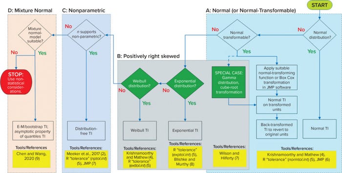
Univariate Data Structure (Fully Observed): When only a single measurement is made per lot (n = 1, release-only data), the data structure is univariate, and all data are fully observed (>LoQ), then apply the decision tree in Figure 1.

Figure 1: Flow diagram for univariate data (fully observed); TI = tolerance interval, E-M = expectation-maximization.

Normal or Normal-Transformable: Normal distribution is the most common, well-characterized distribution, and it applies to many quality attributes. The univariate normal TI is the simplest type and can be calculated using equations in Section 2.2–2.3 of the book Statistical Tolerance Boxes: Theory, Applications, and Computation (4), the normtol.int function in the R “tolerance” package (5), or the distribution platform in JMP software (6). Cited resources are highlighted in bright yellow boxes at the bottom of Figure 1.

If data are not normal, then determine whether they can be transformed using either the best-fitting continuous distribution in JMP software or through Box-Cox transformation. If so, then the univariate normal TI formula can be applied to the transformed data, and the calculated TI can be back-transformed to revert to the original units of measure.

Positively Right-Skewed: For attributes that are positively right-skewed (e.g., microbial limits, environmental monitoring parameters, and certain impurities), the lognormal and gamma distributions are logical choices. Both distributions fall under the normal-transformable category — hence their inclusion in box a of Figure 1. Lognormal is covered under the step for a normal-transforming function (taking the natural logarithm). The cube-root transformation works particularly well as a normal-transform approximation of gamma-distributed data (7). The calculated TI for either log- or cube-root transformed data can be exponentiated or cubed back to revert to the original units of measure.

Generally, gamma distribution can take on the shape of exponential and Weibull distributions depending on the values of the associated parameters. TIs are not predicated on normal transformation for either distribution, so they are presented separately in box b without overlapping with box a of Figure 1. For exponential distributions, use either the tolerance-package exptol.int function (5) or equations from Section 5.5.3 of the book, Reliability: Modeling, Prediction, and Optimization (8). For Weibull distributions, use either the exttol.int function (5) or equations for generalized pivotal quantities in Section 7.5.2 of (4). The suitability of exponential and Weibull distributions can be compared with that of lognormal or gamma distributions through the best-fitting distribution platform in JMP software. If the data include zero values, note that both exponential and Weibull distributions can handle them; gamma and lognormal distributions cannot.

Nonparametric: When no distribution is assumed, use nonparametric TI methods relying on row-order statistics if the minimum sample size requirement is met (Figure 1, box c). Calculate nonparametric TIs using either the equations for row indices in Section 5 of the book Statistical Intervals: A Guide for Practitioners and Researchers (2), the nptol.int function (5), or the distribution platform in JMP software. Note that when an assumed distribution can be justified, the corresponding parametric approach provides a stronger basis than nonparametric methods.

Mixture-Normal Distributions: If none of the above conditions apply, then the last resort may be the mixture of normal distributions (Figure 1, box d). Chen and Wang described methods for TI based on mixtures of normal populations (9). They use maximum likelihood estimation (MLE) through an expectation-maximization (E-M) algorithm to estimate means and standard deviations as well as the proportion of component-normal distributions. Those estimates are used to calculate TI through bootstrapping.

The applicability of the mixture-normal populations ideally would be advised by an SME. Relying solely on observed data to infer the number and proportion of mixture components can be misleading. If nonnormal data cannot be transformed into normal data, if sample size does not support nonparametric TI, and if the results cannot be modeled adequately as a mixture of normal populations, then the specification might have to be established using nonstatistical considerations.

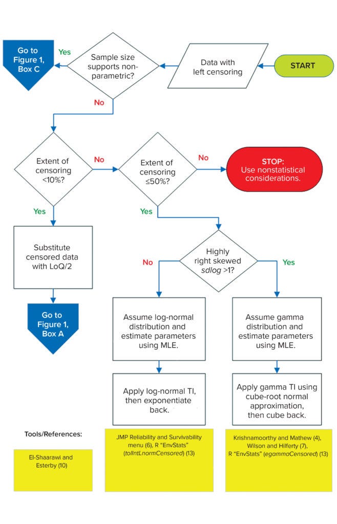
Univariate Data Structure (with Left-Censoring): When some measurements are below LoQ, that is a case of left-censoring, referred to here simply as censoring. When censored data are present, specification setting becomes more complicated than when data are observed fully. Different methods for treating censored data have been described in the vast literature of environmental statistics. The cardinal rule is that such data should not be excluded from calculations. Even though no numerical values can be reported, these data still are informative to analysts, demonstrating the fraction of the data that falls below LoQ. Ignoring that useful information by excluding censored data leads to biased distribution-parameter estimates. Figure 2 summarizes two methods for TI calculation with censored data. If the sample size supports application of a nonparametric TI, then apply the distribution-free TI in box c of Figure 1. Otherwise, proceed with the decision tree in Figure 2.

Figure 2: Flow diagram for univariate data (with left censoring); LoQ = limit of quantitation; MLE = maximum likelihood estimation.

Substitution: Practitioners often substitute censored data with a constant (e.g., ½ × LoQ), but doing so is not recommended because, like exclusion, it leads to biased estimates. However, when the extent of censoring is <10%, the bias will be low (10). With censored values substituted, such data sets are treated as if they had been fully observed, so the normality decision tree and subsequent paths in box a of Figure 1 would be followed as usual. The simplicity of this treatment — preventing the need for more statistically rigorous but more computationally complex methods (see below) — will appeal to many practitioners.

Maximum Likelihood Estimation (MLE): From the literature of environmental statistics comparing different approaches to treat censored data, the consensus is that MLE is the best approach. It assumes an applicable parametric distribution for the population from which data were drawn. Then the likelihood for both observed data (based on the probability density function) and censored data (based on the cumulative density function evaluated at the reporting limit) is maximized to estimate the distribution parameters. MLE is mathematically complex to implement, but available computing tools can help.

If the extent of data censoring is 10–50%, and a data set is not too highly right-skewed (standard deviation of log-transformed data, sdlog < 1), then use the MLE method with lognormal distribution. Some studies show that for this distribution, an extent of censoring even as high as 80% introduces only low (<10%) parameter-estimate bias (11, 12). However, because applicable distribution is inferred from the data, and sample sizes typically are limited (n < 30), such assessment becomes unreliable if the data are highly censored. To be conservative, a 50% censoring maximum threshold is used in this proposed framework.

R packages such as EnvStats can be used to output both geometric mean (meanlog) and geometric standard deviation (sdlog) estimates as well as the resulting TIs directly through the tolIntLnormCensored function (13). Life Distribution and Fit Parametric Survival platforms under the “Analyze > Reliability and Survival” menu in JMP software also can be used to generate meanlog and sdlog. The resulting estimates are substituted into a univariate normal TI formula to calculate lognormal TI, which upon exponentiation yields TI in the original units of measure.

When the extent of censoring is 10–50%, but a data set is highly right-skewed (sdlog > 1), then using MLE assuming lognormal distribution would lead to unrealistic upper statistical limits, especially for small sample sizes (n < 30). For such cases, a technical guide from the US Environmental Protection Agency recommends an alternative MLE method using gamma distribution (14).

To help readers understand the gamma TI approach, some mathematical notation and symbols are introduced here: Suppose Y ~ Gam(k,θ), where Y is the gamma-distributed drug attribute, and k and θ are the shape and scale parameters, respectively. The cube-root transformation (7) of the gamma distribution is approximately normal, with mean (μ) and variance (σ²) that are functions of gamma parameter estimates k ̂ and θ ̂ — see Section 7.3.1 of (4). Gamma distribution is not included in the “Reliability and Survival” JMP menu. The egammaCensored function in EnvStats (13) can be used instead to output k ̂ and θ ̂, which are then applied in calculating μ ̂ and σ ̂ ². The TI of the cube-root transformed data — TI_Y⅓ — is calculated by the univariate normal TI formula using μ ̂ and σ ̂ ². Cubing back TI_Y⅓ yields the gamma TI for the censored data.

If the extent of censoring is >50%, then MLE methods can yield unreliable parameter estimates. Analysts can try those methods using either lognormal or gamma distributions. If the derived TI is inconsistent with observed data (e.g., too much white space, does not fully bracket all observations, and so on), then practitioners may have to use nonstatistical considerations for establishing specification limits.

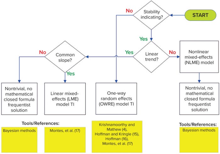
Hierarchical Data Structure: In most cases, data will come from a combination of single measurements per lot (n_i = 1, release only) and multiple measurements over time per lot (n_i ≥ 1, stability data), where i is the ith lot. For this hierarchical data structure, with all data fully observed (above LoQ), follow the decision tree in Figure 3. Note that working with left-censored hierarchical data is outside the scope of this framework.

Figure 3: Flow diagram for hierarchical data; LME = linear mixed-effects; OWRE = oneway random effects; NLME = nonlinear mixed-effects.

Non–Stability-Indicating: If the nature of a quality attribute is not stability-indicating (no change over time), then follow the one-way random effects (OWRE) model TI path in Figure 3. For such attributes, the stability measurements from a lot can be assumed to be replicates for that lot. When there is process variability across lots, the measurements within each lot are correlated, and their degree of correlation increases as lot-to-lot variation increases. An appropriate statistical model to take that correlation into consideration is the OWRE design, termed as such because one factor (lot) is randomly sampled from the population, with replicate measurements for each lot.

Hoffman and Kringle present methods for two-sided and one-sided TIs for OWRE models (15, 16). The methods use closed-form formulas consisting of variance components, lot statistics, and F distribution quantiles. Section 5 of (4) provides methods using a generalized confidence interval concept that is simulation-based. Montes et al. present a closed-form TI formula similar to Hoffman’s, but with R code supplied for easy implementation (17).

Stability-Indicating: If a quality attribute is stability-indicating (changes over time), then follow the linear trend decision-tree path of Figure 3. The simplest type of change over time is linear (zero-order kinetics), which covers most attributes encountered in pharmaceutical settings. Additionally, for well-characterized and sufficiently controlled manufacturing processes, manufactured lots should have a common degradation pattern (slope), even if their release values vary. The linear mixed-effects (LME) model applies for such cases. Having both a random effect manifested as lot-to-lot variation at release (intercepts) and a fixed effect manifested as a common slope among stability lots renders a model as mixed-effects. The trend is assumed to be linear, hence the name: linear mixed-effects model.

Sharma and Mathew present a TI method for LME models based on a small-sample asymptotic procedure, but the computation is highly complex (18). Montes et al. cover LME TI with relatively simple closed-form formulas included as R code for easy implementation (17). The LME TI formula is evaluated at either time zero to set release limits or at shelf life to set stability specification limits. The paper demonstrated that combining release and stability data provides better statistical properties than using stability data alone. The latter practice essentially ignores information from available release data.

A single LME TI formula to set release limits and stability specification not only ensures consistency between the two, but also offers practical advantages. The more efficient statistical modeling lends to easier coding than analyzing release and stability data separately and then linking the results together with some ad hoc adjustment. The common slope assumption in the LME model is justified from a manufacturing process-control perspective. Meeting that assumption mathematically simplifies construction of TI for hierarchical data structures with linear trends.

For situations in which a varying-slope assumption applies (rather than a common slope) as justified by SMEs, no published closed-formula solution is yet available using a classical frequentist approach. A Bayesian approach might be able to handle the additional complexity of slope heterogeneity in such cases. SMEs need to specify the range of acceptable slope variation that can be incorporated into the prior distribution of the slope parameter.

If the change over time for hierarchical data is nonlinear, then the nonlinear mixed-effects (NLME) model applies. The nlreg.tol function in the tolerance package calculates TI for nonlinear regression, but it does not account for the random-lot effect (5). The TI for NLME models is nontrivial, and no available tools use the classical frequentist method for that. A Bayesian approach can be attempted.

A Decision Framework
The framework herein can be used for choosing the type of TI for setting specification limits based on data from manufactured drug lots. The determining factors are assumed data distribution, structure of the data, nature of the quality attribute being specified, and whether left censoring is present in the data. Refer to the computing resources cited for guidance.

References
1 ICH Q6A. Specifications: Test Procedures and Acceptance Criteria for New Drug Substances and New Drug Products: Chemical substances. US Fed. Reg. 65(251) 2000: 83041–83063; https://database.ich.org/sites/default/files/Q6A%20Guideline.pdf.

2 Meeker WQ, Hahn GJ, Escobar LA. Statistical Intervals: A Guide for Practitioners and Researchers (Second Edition). John Wiley & Sons, Inc.: Hoboken, NJ, 2017.

3 Dong X, Tsong Y, Shen M. Statistical Considerations in Setting Product Specifications. J. Biopharm. Stat. 25(2) 2014: 280–294; https://doi.org/10.1080/10543406.2014.972511.

4 Krishnamoorthy K, Mathew T. Statistical Tolerance Regions: Theory, Applications, and Computation. John Wiley & Sons, Inc.: Hoboken, NJ, 2009.

5 Young DS. Tolerance: An R Package for Estimating Tolerance Intervals. J. Statist. Software 36(5) 2010: 1–39; https://doi.org/10.18637/jss.v036.i05.

6 JMP Version 17. SAS Institute Inc.: Cary, NC, 2023.

7 Wilson EB, Hilferty MM. The Distribution of Chi-Square. Proc. Nat. Acad. Sci. 17, 1931: 684–688.

8 Blischke WR, Murthy DNP. Reliability: Modeling, Prediction, and Optimization. Wiley: New York, NY, 2000.

9 Chen C, Wang H. Tolerance Interval for the Mixture Normal Distribution. J. Qual. Technol. 52(2) 2020: 145–154; https://doi.org/10.1080/00224065.2019.1571338.

10 El-Shaarawi AH, Esterby SR. Replacement of Censored Observations By a Constant: An Evaluation. Water Res. 26(6) 1992: 835–844; https://doi.org/10.1016/0043-1354(92)90015-V.

11 Huybrechts T, et al. How To Estimate Moments and Quantiles of Environmental Data Sets with Non-Detected Observations? A Case Study on Volatile Organic Compounds in Marine Water Samples. J. Chromatog. A 975(1) 2002: 123–133; https://doi.org/10.1016/S0021-9673(02)01327-4.

12 Suzuki Y, Tanaka N, Akiyama H. Attempt of Bayesian Estimation from Left-Censored Data Using the Markov Chain Monte Carlo Method: Exploring Cr(VI) Concentrations in Mineral Water Products. Food Safety 8(4) 2020: 67–89; https://doi.org/10.14252/foodsafetyfscj.D-20-00007.

13 Millard SP. EnvStats: An R Package for Environmental Statistics (Second Edition). Springer: New York, NY, 2013.

14 Singh A, Singh AK. EPA/600/R-07/041: ProUCL Version 5.1.002 Technical Guide. US Environmental Protection Agency: Atlanta, GA, 2015; https://www.epa.gov/sites/default/files/2016-05/documents/proucl_5.1_tech-guide.pdf.

15 Hoffman D, Kringle R. Two-Sided Tolerance Intervals for Balanced and Unbalanced Random Effects Models. J. Biopharm. Statist. 15(2) 2005: 283–293; https://doi.org/10.1081/bip-200048826.

16 Hoffman D. One-Sided Tolerance Limits for Balanced and Unbalanced Random Effects Models. Technometrics 52(3) 2010: 303–312; https://www.jstor.org/stable/27867252.

17 Montes RO, Burdick RK, Leblond DJ. Simple Approach to Calculate Random Effects Model Tolerance Intervals to Set Release and Shelf-Life Specification Limits of Pharmaceutical Products. PDA J. Pharm. Sci. Technol. 73(1) 2019: 39–59; https://doi.org/10.5731/pdajpst.2018.008839.

18 Sharma G, Mathew T. One-Sided and Two-Sided Tolerance Intervals in General Mixed and Random Effects Models Using Small-Sample Asymptotics. J. Am. Statist. Assoc. 107(497) 2012: 258–267; https://doi.org/10.1080/01621459.2011.640592.

Richard O. Montes, PhD, is director of CMC statistics at Alnylam Pharmaceuticals, Inc.,
675 West Kendall Street, Cambridge, MA 02142; [email protected].